Wegener I. Complexity Theory. Exploring the Limits of Efficient Algorithms

Подождите немного. Документ загружается.

14.4 Branching Programs and Space Bounds 209

tape cells are suﬃcient to evaluate the left subformula. This result is stored

in one cell, and along with the at most d − 1 tape cells needed to evaluate

the right subformula, at most d tape cells are required. In the end only two

tape cells are being used, and after evaluation of the root, only one tape cell

is being used. 

If the given circuit family is uniform, then the information about a gate can

be computed in space O(log 2

d(n)

)=O(d(n)). So in this case even a uniform

Turing machine can get by with space O(d

∗

(n)).

There are close connections between circuit families and non-uniform

Turing machines, and between Turing machines and uniform families

of circuits. Circuit size is polynomially related to computation time,

and circuit depth is polynomially related to space.

14.4 Branching Programs and Space Bounds

Now we want to introduce a non-uniform model of computation, the size of

which characterizes the space used by non-uniform Turing machines asymp-

totically exactly. This model of computation has roots not only in complexity

theory but also as a data structure for Boolean functions. For this reason there

are two names commonly given to this model: branching program and binary

decision diagram (abbreviated BDD).

A branching program works on n Boolean variables x

,...,x

and has only

two types of elementary commands, which are represented as the vertices of

a graph. A branching (or decision) vertex v is labeled with a variable x

and

has two out-going edges: one labeled 0, the other labeled 1. If v is reached

in a computation, then the edge leaving v corresponding to the value of x

used to arrive at the next vertex. An output vertex w is labeled with a value

c ∈{0, 1} and has no out-going edges. If w is reached, then the computation

is complete and the value c is given as output. A branching program is a

directed acyclic graph consisting of branching vertices (also called internal

vertices) and output vertices (also called sinks).

Each vertex v in a branching program realizes a Boolean function f

the following way. To compute f

(a)westartatvertexv and carry out the

commands at each vertex until we reach a sink. For branching programs there

are two obvious complexity measures. The length of a branching program is

the length of the longest computation path in the branching program and is

a measure of the worst-case time required to evaluate the function. The size

of a branching program is the number of vertices, and the branching program

complexity BP(f) of a Boolean function f is deﬁned as the minimal size of

a branching program that computes f. This is the complexity measure that

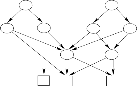
we will be interested in here. Figure 14.4.1 contains a branching program the

input vertices of which realize the two output bits for the addition of three

bits. To make the diagram more readable we have included two 1-sinks.

210 14 The Complexity of Non-uniform Problems

101

Fig. 14.4.1. A branching program for the addition of three bits.

So why is there a tight connection between the size of branching pro-

grams and the space required by non-uniform Turing machines? To evaluate

it is suﬃcient to remember the currently reached vertex. On the other

hand, a branching program can directly simulate the conﬁguration graph of a

space-bounded Turing machine used in the proof of Theorem 14.2.2. We will

formalize this in the theorem below, using BP

∗

) to represent the larger of

BP(f

)andn, and letting s

∗

(n)=max{s(n), log n} just as before.

Theorem 14.4.1. The decision problem A

corresponding to f =(f

) can

be solved by a non-uniform Turing machine in space O(log BP

∗

)).

Proof. For help on inputs of length n we use a description of a branching

program G

of minimal size for f

. This description includes a list of the

vertices, where each vertex is described by its type (inner vertex or sink),

its number, and its internal information. For a sink the latter consists of the

value that is output by the sink, and for an inner vertex it consists of a

triple including the index of the variable to be processed, the index of the

0-successor, and the index of the 1-successor. Furthermore, we will always

let the vertex representing f

have index 1. In this way each of the BP(f

)

vertices has a description of length O(log BP

∗

)). We use the work tape

to remember the current vertex, so at the beginning of the computation it

contains the number 1. If a sink is reached, then we make the correct decision

and stop the computation. Otherwise we search for the value of the variable to

be processed on the input tape. After that the new current vertex is known,

namely the x

-successor. We look for its information on the help tape and

update the current vertex index on the work tape. 

Theorem 14.4.2. An s(n)-space bounded Turing machine can be simulated

by a branching program of size 2

O(s

∗

(n))

Proof. We already know that the number of diﬀerent conﬁgurations of the

Turing machine on an input of length n is bounded by 2

O(s

∗

(n))

. The branching

14.5 Polynomial Circuits for Problems in BPP 211

program G

has a vertex for each of the conﬁgurations that is reachable from

the start conﬁguration. Accepting conﬁgurations are 1-sinks and rejecting

conﬁgurations are 0-sinks. An inner vertex for conﬁguration K is labeled with

the variable x

that is being read from the input tape in conﬁguration K.

The 0-child of this vertex is the conﬁguration that is reached in one step

from K if x

= 0. The 1-child is deﬁned analogously. Since we only consider

Turing machines that halt on all inputs, the graph is acyclic and we have a

branching program. The Boolean function describing the acceptance behavior

of the Turing machine on inputs of length n is realized by the vertex labeled

with the initial conﬁguration. 

What changes if the given Turing machine is non-uniform and the help

has length h(n)? The number of conﬁgurations and therefore the size of

the simulating branching program grows by a factor of h(n) ≤ 2

log h(n)

This has led to the convention of adding log h(n) to the space used

by a non-uniform Turing machine. Or we could instead deﬁne s

∗∗

(n)=

max{s(n), log n, log h(n)}.Thetermlog n has the same function for

the input tape as the term log h(n) has for the help tape.

Corollary 14.4.3. An s(n)-space bounded non-uniform Turing machine can

be simulated by a branching program of size 2

O(s

∗∗

(n))

. 

These results can be summarized as follows for the “normal” case that

s(n) ≥ log n,BP(f

) ≥ n,andh(n) is polynomially bounded:

Space and the logarithm of the branching program size have the same

order of magnitude.

For a language L ∈

NP, L ∈ P,orL ∈ NTAPE(log n), we can try to show

that L/∈

DTAPE(log n) by proving a superpolynomial lower bound for the

branching program size of the function f

=(f

). This is the most common

line of attack for such results. To this point, such lower bounds for branching

program size grow more slowly than quadratically (see Chapter 16).

14.5 Polynomial Circuits for Problems in BPP

We have already discussed several times that BPP is “not much larger” than

P.ItispossiblethatBPP = P, but this is still an open question. Now we want

to oﬀer some support for the claim that problems in

BPP are not much more

diﬃcult than problems in

P. For a decision problem A ∈ BPP the Boolean

functions f

=(f

) can be computed by circuits of polynomial size. If these

circuits were uniform, then it would follow that

BPP = P. But so far, only

non-uniform circuits for f

have been found. The trick is that for a BPP algo-

rithm we can choose the error-probability to be so low that by the pigeonhole

principle there must be an assignment for the random bits for which the

BPP

212 14 The Complexity of Non-uniform Problems

algorithm makes no mistakes. We will choose this assignment of the random

bits as help for a non-uniform Turing machine which can then be simulated

by circuits as in Sections 14.2 and 14.3.

Theorem 14.5.1. Decision problems A ∈

BPP can be solved by polynomial-

time deterministic non-uniform Turing machines. The Boolean functions

=(f

) have polynomially bounded circuit size.

Proof. Since A ∈

BPP, by Theorem 3.3.6 there is a randomized Turing ma-

chine M that decides A in polynomial time p(n) with an error-probability

bounded by 2

−(n+1)

. Now consider a 2

× 2

p(n)

-matrix such that the rows

represent the inputs of length n and the columns represent the assignments

of the random vector r. Since in p(n) steps at most p(n) random bits can be

processed, we can restrict our attention to random vectors of length p(n). Po-

sition (x, r) of the matrix contains a 1 if M on input x with random vector r

is incorrect. Otherwise the matrix entry is 0. Since the probability of an error

is bounded by 2

−(n+1)

, each row contains at most 2

p(n)−(n+1)

1’s. The total

number of 1’s in the matrix is then bounded by 2

p(n)−1

By the pigeonhole

principle at least half of the columns must contain only 0’s. We choose one of

the corresponding random vectors r

∗

as help h(n) for a non-uniform Turing

machine M



. The Turing machine M



simulates M using h(n)=r

∗

where M

uses random bits. So M



is deterministic and makes no errors. Furthermore,

the runtime of M



is bounded by p(n). 

For

BPP algorithms with suﬃciently small error-probability there is a

golden computation path that works for all inputs of the same length. This

computation path can be eﬃciently simulated – if it is known. The diﬃculty

of derandomizing

BPP algorithms is the diﬃculty of ﬁnding this golden com-

putation path. Note that is not because there are so few of them: If the

error-probability of the

BPP algorithm is reduced to 2

−2n

, then the fraction

of golden computation paths among all computation paths is at least 1− 2

−n

14.6 Complexity Classes for Computation with Help

Before we ask whether NP algorithms can be simulated by circuits of polyno-

mial size, as

BPP algorithms can be, we want to investigate more closely the

complexity classes that arise from non-uniform Turing machines. In polyno-

mial time only a polynomially long help can be read. So we will only allow

polynomially long help. Furthermore, we will restrict ourselves to determin-

istic and nondeterministic polynomial-time computations. Generalizations of

both of these aspects are obvious.

Deﬁnition 14.6.1. The complexity class

P/poly contains all decision prob-

lems that can be decided in polynomial time by non-uniform deterministic

Turing machines with polynomially long help.

NP/p oly is deﬁned analogously

using nondeterministic Turing machines.

14.6 Complexity Classes for Computation with Help 213

The following characterization of P/poly follows from earlier results.

Corollary 14.6.2.

P/poly contains exactly those decision problems A for

which f

=(f

) has polynomially bounded circuit size.

Proof. Theorem 14.3.1 says that the existence of polynomial-size circuits for

=(f

) implies that A ∈ P/poly. Theorem 14.2.1 and the remarks at the

beginning of Section 14.3 provide the other direction of the claim. 

Now we can also present Theorem 14.5.1 in its customary brief form:

Corollary 14.6.3.

BPP ⊆ P/poly. 

The

= P-question has a non-uniform analogue, namely the NP/poly

P/poly-question. In order to get a better feeling for the class NP/poly we will

present a characterization in terms of circuits for this class as well. Since

NP expresses the use of an existential quantiﬁer over a polynomially long

bit vector, we must give our circuits the possibility of realizing existential

quantiﬁers.

Deﬁnition 14.6.4. A nondeterministic circuit C is a circuit for which the

inputs are partitioned into input variables x and nondeterministic variables

y. Each gate G in such a circuit computes the function f

: {0, 1}

|x|

→{0, 1}

deﬁned such that f

(a)=1if and only if there is a b ∈{0, 1}

|y|

such that

gate G computes the value 1 when the values of the x-variables are given by

a and the values of the y-variables are given by b.

Theorem 14.6.5.

NP/p oly contains exactly those decision problems A for

which the Boolean functions f

=(f

) have nondeterministic circuits of

polynomial size.

Proof. First suppose that A ∈

NP/p oly. We can assume that we have a non-

uniform nondeterministic Turing machine M for A that on inputs of length n

takes exactly p(n) steps for some polynomial p. The circuit C

that simulates

M on inputs of length n contains, in addition to the n input variables, constant

inputs representing the help for M for inputs of length n, and nondeterministic

input variables that describe the nondeterministic choices of M. With respect

to this longer input, M works deterministically and can be simulated by a

polynomial-size circuit. Considered as a nondeterministic circuit, with the

appropriate partitioning of the inputs, this circuit computes the function f

Now suppose we have nondeterministic circuits C =(C

)forf

=(f

The non-uniform Turing machine M receives as help for inputs of length n

a description of the circuit C

. M then randomly generates values for the

nondeterministic inputs and simulates C

on the extended input vector. Thus

M decides A in polynomial time. 

214 14 The Complexity of Non-uniform Problems

14.7 Are There Polynomial Circuits for all Problems in

NP?

Since BPP ⊆ P/poly, one can ask if it is also (or even) the case that

NP ⊆ P/poly. This would not lead directly to eﬃcient algorithms for NP-

equivalent problems, but we would at least have a better idea about what

makes them diﬃcult. Since polynomial reductions can be simulated by cir-

cuits of polynomial size, either all

NP-complete problems are in P/poly,or

P/poly contains no NP-complete problems. Since P ⊆ P/poly,wecan’thopeto

prove that

NP ⊆ P/poly. On the other hand, we believe that NP is so much

farther from

P than BPP is that NP can’t be a subset of P/poly.Wealready

know the way out of this situation. We will show that one of our well-founded

complexity theoretic hypotheses is false if

NP ⊆ P/poly.Inthiscaseitisthe

hypothesis Σ

= Σ

. Expressed diﬀerently, NP can only be a subset of P/poly

if the polynomial hierarchy collapses to the second level, namely to Σ

For the proof of this claim it suﬃces to show for some problem A ∈

that

A ∈

P/poly ⇒ Σ

= Σ

The obvious choice for A is some

NP-complete problem. The inputs of A have

to be coded in binary, but this doesn’t aﬀect the complexity with respect

to the usual descriptions of the problems we have considered. So what

NP-

complete problem should we choose? Based on our experience, the standard

choice would be

Sat or 3-Sat. This choice works here as well. But we will see

in our proof that it is only important to choose an

NP-complete problem with

the following property:

Deﬁnition 14.7.1. A decision problem is called polynomially self-reducible

if it is Turing reducible to itself in such a way that all the queries made by the

reduction are to instances of shorter length than the instance to be decided.

Later we will see how this property gets used. First we show two examples

NP-complete problems that are polynomially self-reducible.

Lemma 14.7.2.

Sat and Clique are polynomially self-reducible.

Proof. For

Sat we can decide instances with no variables directly in polyno-

mial time. Otherwise we choose a variable x that occurs in our

Sat instance

ϕ, form instances ϕ

= ϕ

|x=0

and ϕ

= ϕ

|x=1

, and query the subprogram for

Sat on these two shorter instances. The formula ϕ is satisﬁable if and only if

at least one of ϕ

and ϕ

is satisﬁable.

For

Clique we can decide instances with n =1ork = 1 directly in

polynomial time. So let (G, k) be an instance of

Clique with n, k ≥ 2. We

select a vertex v from G with minimal degree. If the degree of this vertex

is n − 1, then we have a complete graph and can again decide about the

instance (G, k) directly. Otherwise we construct two graphs: G

is the result

of removing v from G,andG

is the subgraph of G containing only those

14.7 Are There Polynomial Circuits for all Problems in NP? 215

vertices connected to v by an edge. By our choice of v, both G

and G

have

a shorter description than G.Wequery

Clique about (G

,k)and(G

,k− 1),

and we accept only if at least one of these queries is accepted by

Clique.This

decision is correct since G has a clique of size k if and only if there is a clique

of size k that doesn’t use vertex v or a clique of this size that contains v.But

the second case is equivalent to the existence of a clique of size k − 1among

the neighbors of v. 

For a polynomially self-reducible problem A we will let M

denote

a polynomial-time Turing machine that decides A with queries to an A-

subprogram for shorter instances of A. This same Turing machine can also be

used with an oracle for a diﬀerent decision problem B.Inthiscasewewill

let L(M

,B) denote the language accepted by M

with oracle B. Finally, for

C ⊆{0, 1}

∗

we let C

≤n

denote the set of all x ∈ C with |x|≤n. Now we are

ready to prove a technical lemma that allows us to draw consequences from

the self-reducibility of A.

Lemma 14.7.3. For a polynomially self-reducible decision problem A and a

language B ⊆{0, 1}

∗

if L(M

,B)

≤n

= B

≤n

, then A

≤n

= B

≤n

Proof. We prove the lemma by induction on n.Forn = 0 the only allowed

input is the empty string. Since there are no shorter strings, the subprogram

for M

cannot be called, and so A

≤0

= L(M

,A)

≤0

= L(M

,B)

≤0

= B

≤0

Now suppose that L(M

,B)

≤n+1

= B

≤n+1

.ThenL(M

,B)

≤n

= B

≤n

,so

by the inductive hypothesis A

≤n

= B

≤n

. We must show that A

≤n+1

= B

≤n+1

For a string of length n + 1 the Turing machine queries the subprogram only

about strings y with |y|≤n. So it doesn’t matter if the subprogram is deciding

A, A

≤n

, B

≤n

,orB since these are all the same on strings of length up to n.

It follows that

≤n+1

= L(M

,A)

≤n+1

= L(M

,B)

≤n+1

= B

≤n+1

with the last equality following from our assumption. This proves the lemma.



In what follows let A be a polynomially self-reducible

NP-complete set like

the ones we encountered in Lemma 14.7.2. Once again let M

be a polynomial-

time Turing machine that decides A with the help of queries to shorter in-

stances of A. Our goal is to show that if A ∈

P/poly, that is, if there exist

polynomial-size circuits C =(C

)forf

=(f

), then Σ

= Σ

. It is impor-

tant that instances of A be coded in binary. Circuits only work on inputs of

a ﬁxed length. For our purposes, it would be nice to have circuits that could

process all instances of length up to m. So we will consider a circuit with

input length m+ log m, such that the ﬁrst log m input bits code a number

i ∈{1,...,m} and the original circuit C

is then simulated on the next i

input bits. It is easy to construct such a family of circuits C

∗

=(C

∗

)from

216 14 The Complexity of Non-uniform Problems

the family C =(C

) in polynomial time and in such a way that the new cir-

cuits also have polynomial size. Now if a subprogram is called that simulates

circuit C

for an arbitrary i ≤ m, then we can replace this subprogram with a

program that simulates C

∗

instead. Within the subprogram we ﬁrst compute

a suitable input for C

∗

. From this it follows that L(M

∗

)

≤m

= A

≤m

Said diﬀerently: For instances x of length i, x ∈ L(M

∗

) if and only if

(x) = 1. Based on this preliminary discussion we will now show how from

the assumption that there are polynomial-size circuits for the

NP-complete

problem A, it follows that languages in Σ

are already contained in Σ

Theorem 14.7.4. If NP ⊆ P/poly, then Σ

= Σ

Proof. Let A be a polynomially self-reducible NP-complete decision problem.

NP ⊆ P/poly, then there is a circuit family C =(C

)forA of polynomial

size that computes f

=(f

). We will also make use of the polynomial-size

circuits C

∗

as described above.

Now let L ∈ Σ

. By Theorem 10.4.3 there is an ∃∀∃-representation for L

with a polynomial-time predicate. We can turn this into an ∃∀-representation

with an

NP predicate. Since A is NP-complete, we can reduce the NP predicate

to A with a polynomial reduction f. Thus for some polynomial p we have

L = {x: ∃y |y|≤p(|x|) ∀z |z|≤p(|x|): f(x, y, z) ∈ A} .

The length of f(x, y, z) is bounded by q(|x|) for some polynomial q. We claim

that L can be characterized in the following way, where p



is a suitable poly-

nomial.

L = {x: ∃(C, y)with|C|≤p



(|x|)and|y|≤p(|x|)

∀(w, z)with|w|≤q(|x|)and|z|≤p(|x|)

C describes a circuit with size polynomial in |x|

for inputs of length at most q(|x|),

w ∈ L(M

,C) ⇔ C

|w|

(w)=1, and

C computes the value 1 for f (x, y, z)} .

In order for this to be a Σ

characterization, the three properties must be

checkable in polynomial time. For the ﬁrst property this is clearly true for the

usual description of circuits. For the second property this follows since M

polynomially time-bounded, we can replace subprogram calls with simulations

of C, and the evaluation of circuits can be done in polynomial time. Since f

can be computed in polynomial time, we can also check the third property in

polynomial time.

Finally, we show that this characterization of L is correct. First let x ∈ L.

For our circuit C we choose a circuit of polynomial size that checks for (b, a) ∈

{0, 1}

log q(|x|)

×{0, 1}

q(|x|)

whether the preﬁx of a of length bin(b) belongs to

A.Hereweareusingbin(b) to represent the number from {1,...,q(|x|)} that

is represented by b. We consider C as a circuit for inputs a with |a|≤q(|x|)

14.7 Are There Polynomial Circuits for all Problems in NP? 217

that checks for membership in A. The correctness of the second condition

follows from our preliminary discussion. By Lemma 14.7.3, C accepts exactly

those instances that belong to A, and thus C accepts f(x, y, z).

For the other direction we assume that x satisﬁes the logical character-

ization given above. By Lemma 14.7.3 the second condition implies that C

accepts inputs (b, a) ∈{0, 1}

log q(|x|)+q(|x|)

if and only if the preﬁx of a spec-

iﬁed by b belongs to A. From the third condition it follows that f(x, y, z) ∈ A.

So x ∈ L now follows from the previous characterization of L.Thisprovesthe

theorem. 

The results in Corollary 14.6.3 and Theorem 14.7.4 can be interpreted

as saying that

NP presumably contains problems that are more diﬃcult (with

respect to circuit size) than the problems in

BPP.Inparticular,NP is probably

not contained in

BPP.

Communication Complexity

15.1 The Communication Game

The goal of complexity theory is to estimate the minimal resources needed to

solve algorithmic problems. The lower bounds we have proven so far depend

on complexity theoretic hypotheses or are with respect to specialized scenarios

like the black box scenario. In this chapter and the next we will prove lower

bounds for one resource without complexity theoretic assumptions but under

the condition that some other resource is suﬃciently restricted, i.e., so-called

trade-oﬀ results. Among these will be results in Chapter 16 giving size lower

bounds for bounded-depth circuits and or for bounded-length branching pro-

grams. Probably the earliest results of this type were about the area A and

the parallel computation time T of VLSI circuits (see also Section 15.5). For

certain functions f =(f

), Thompson (1979) showed that the product of area

and the square of the runtime must grow asymptotically at least as fast as n

expressed formally: AT

= Ω(n

). This means that area and runtime cannot

both be small. Yao (1979) ﬁltered out the core of the ideas used in the proof

of these bounds and separated it from the speciﬁc applications. Out of this

came the theory of communication complexity, which is based on the following

communication game.

Alice and Bob cooperate to evaluate a function f : A × B → C based on

distributed information about the input. They need to compute f(a, b)for

a ∈ A and b ∈ B. Alice knows a but not b, and Bob knows b but not a.How

the input is distributed among Alice and Bob is part of the question. The

goal is to come to a point where both Bob and Alice know that both of them

know the value of f(a, b). Communication complexity only deals with the case

that A, B,andC are ﬁnite. In most of our examples we will be investigating

Boolean functions with a single output, that is, the case where A = {0, 1}

B = {0, 1}

,andC = {0, 1}.

The communication game places an emphasis on the information ex-

changed between Alice and Bob. The goal is to minimize the worst-case (with

respect to the various inputs (a, b)) number of bits that Alice and Bob ex-