Yang X.-S. Introductory Mathematics for Earth Scientists

Подождите немного. Документ загружается.

190 Chapter 13. Geostatistics

By expanding these equations, we have

na + b

i=1

, (13.37)

and

i=1

+ b

i=1

, (13.38)

which form a system of linear equations for a and b, and it is straight-

forward to obtain the solutions as

a =

[

i=1

− b

i=1

] = ¯y − b¯x, (13.39)

b =

i=1

− (

i=1

)(

i=1

)

i=1

− (

i=1

)

, (13.40)

where

¯x =

i=1

, ¯y =

i=1

. (13.41)

If we use the following notations

i=1

, K

i=1

, K

i=1

, K

i=1

, (13.42)

then the above equations for a and b become

a =

− K

− (K

)

, b =

− K

− (K

)

. (13.43)

The residual error is deﬁned by



= y

− (a + bx

), (13.44)

whose sample mean is given by



i=1



− a − b

i=1

= ¯y − a − b¯x = 0. (13.45)

The sample varia nce S

n − 2

i=1

− (a + bx

)]

, (13.46)

where the factor 1/(n −2) comes from the fact that two constraints are

needed for the best ﬁt, and the residuals therefore have n − 2 degrees

of freedom.

13.5 Correlation Coefficient 191

13.5 Correlation Coeﬃcient

The co rrelation coeﬃcient r

x,y

is a very useful parameter for ﬁnding

any potential relationship between two sets of data x

and y

for two

random variables x and y, respectively. For a set of n data points

, y

), the correlatio n c oeﬃcient can be calculated by

x,y

i=1

−

i=1

− (

i=1

)

][n

i=1

− (

i=1

)

]

, (13.47)

x,y

− K

(nK

− K

)(nK

− K

)

, (13.48)

where K

i=1

If the two variables are independent, then r

x,y

= 0, which means

that there is no correlation between them. If r

x,y

= 1, then there

is a linear relatio nship between these two variables. r

x,y

= 1 is an

increasing linear relationship where the increase of one variable will

lead to increase of another. r

x,y

= −1 is a decreasing relationship

when one increases while the other decreases.

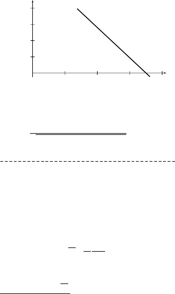
Example 13.4: Let us try to estimate the b-value in the Gutenberg-

Richter law using the da ta from the Southern California Earthquakes. The

numbers of earthquakes from 1987 to 1996 in this region are as follows:

Magnitude above M = 3 4 5 6 7

Total numbers N = 5454 561 64 9 1

In order to ﬁt

log

(N) = a + bM,

we ﬁrst have to convert N into log

N, and we have

= log

N =3.737 2.749 1.806 0 .954 0.

Then, we have

i=1

= 3 + 4 + 5 + 6 + 7 = 25, K

i=1

= 9.246,

i=1

= 3

= 135, K

i=1

= 25 .694,

and K

i=1

= 36.961. Therefore, we have

a =

− K

− (K

)

135 × 9.246 − 25 × 36.961

5 × 135 − 25

≈ 6.4837,

and

b =

− K

− (K

)

5 × 36.961 − 25 × 9.246

5 × 135 − 25

≈ −0.9269.

192 Chapter 13. Geostatistics

2 4 6 8

log

(N)

log

(N) = a + bM

Figure 13.3: Estimating b-value by the best ﬁt to data.

Finally, the correlation coeﬃcie n t deﬁned by (13.48) becomes

r =

5 × 36.961 − 25 ×9.246

(5 × 135 − 25

)(5 × 25.694 − 9.246

)

≈ −0.9997.

This indeed implie s a very strong correlation. The best ﬁt relationship

be c omes log

(N) = 6.4837 − 0.9269M (see Fig. 13.3).

There are many important techniques in geo statistics. Fo r example,

kriging is a very important tool for analysing the data with spatial

correlation and it will provide a good prediction for missing data and

interpolation. Interested readers can refer to mor e advanced literature

13.6 Brownian Motion

Einstein provided in 1905 the ﬁrst theory of Brownian motion of spher-

ical particles suspended in a liquid, which can be written, after some

lengthy calculations, as

∆

3πµa

, (13.49)

where a is the ra dius of the spher ical particle, and µ is the viscosity of

the liquid. T is the absolute temperature, and t is time. k

= R/N

is Boltzmann’s c onstant where R is the universal gas constant and N

is Avogadro’s constant.

∆

is the mean square of the displac e ment.

For example, Yang, X. S., Mathematical Modelling for Earth Sciences, Dunedin

Academic, (2008).

13.6 Brownian Motion 193

Langevin in 1908 pr e sented a very instructive but much simpler

version of the theory. If u is the displacement, and ξ =

is the speed

at a given instant, then the kinetic energy of the motion should be equal

to the average kinetic energy

T .

That is

T, where m

is the mass of the particle. The spherical particle moving at a velocity

of ξ will experience a visco us resistance equal to −6πµaξ = −6πµa

according to Stokes’ law. If F (t) is the complementary force acting

on the particle at the insta nt so as to maintain the agitation of the

particle, we have, according to Newton’s second law

= −6πµa

+ F. (13.50)

Multiplying both sides by u, we have

= −6πµau

+ F u. (13.51)

Since (u

)

/2 = uu

or u

)

−(

)

d(u

)

−ξ

we have

d(u

)

− mξ

= −3πµa

d(u

)

+ F u, (13.52)

where we have used uu

= (u

)

/2. If we consider a large number of

identical particles and take the average, we have

d(u

)

− m

= −3πµa

d(u

)

F u, (13.53)

where () means the average. Since the average of F u = 0 due to the

fact that the force is ra ndom, tak ing any signs and directions. Let

Z =

d(u

)/dt, we have

+ 3πµaZ = k

T, (13.54)

where we have used m

= k

T discussed earlier. This equation is

now known as Langevin’s equation. It is a linear ﬁrst-order diﬀerential

equation. Its general so lution can easily be found using the method

discussed in the chapter on diﬀerential equations

= Ae

−t/τ

+ k

3πµa

, τ =

6πµa

, (13.55)

Here Langevin considered only one direction. For three directions, the kinetic

energy becomes

T , thus there is a factor 3. This means that equation (13.59)

should be u

= 6Dt.

194 Chapter 13. Geostatistics

where A is the constant to be deter mined. For the Brownian motion

to be observable, t must be reasonably larger tha n the characteristic

time τ ≈ 10

−8

seconds, which is often the case. So the ﬁrst term

will decr e ase exponentially and becomes negligible when t > τ in the

standard timescale of our interest. Now the solution becomes

Z =

d(u

)

= k

3πµa

. (13.56)

Integrating it with respect to t, we have

= k

3πµa

, (13.57)

which is Einstein’s formula fo r Brownian motion. Furthermore, the

Brownian motion is essentially a diﬀusion process, and the diﬀusion

coeﬃcient D can be deﬁned as

D =

6πµa

, (13.58)

so that we have

= 2Dt. (13.59)

This suggests that larg e particles diﬀuse more slowly than smaller par-

ticles in the same medium. Mathematically, it is very similar to the

heat conduction process discussed in e arlier chapters.

We know that the diﬀusion coeﬃcient of sugar in water at room

temper ature is D ≈ 0.5 × 10

−9

/s. In 1905, Einstein was the ﬁrst

to estimate the size of sugar molecules using exp e rimental data in his

doctoral dissertation on Brownian motion.

Let us now estimate the size of the sugar molecules. Since k

1.38 × 10

−23

J/K, T = 300 K, and µ = 10

−3

Pa s, we have

a =

6πµD

1.38 × 10

−23

× 300

6π × 10

−3

× 0.5 × 10

−9

≈ 4.4 × 10

−10

m, (13.60)

which means that the diameter is about 8.8×10

−10

m= 8.8 nm. In fact,

Einstein estimated for the ﬁrst time the diameter of a sugar molecule

was 9.9 × 10

−10

m even though the other quantities were not so accu-

rately measured at the time.

From

= 2Dt, we can either estimate the diﬀusion distance fo r a

given time or estimate the timescale for a given length. For a sugar cube

in a cup of water to dissolve completely to form a solution of uniform

concentration (without stirring), the time taken will be t = d

/2D,

where d =

is the size of the cup. Using d = 10 cm= 0.1 m and

D = 0.5 × 10

−9

/s, we have t = 0.1

/(2 × 0.5 × 10

−9

) ≈ 1 × 10

seconds, which is about 3 months. This is too slow; that is why we

always try to stir a cup of tea or coﬀee.

Chapter 14

Numerical Methods

The beauty of an analytical solution to a problem is that it is accu-

rate and often provides some insight into the main process of interest.

However, in most applications, no explicit forms of analytical solutions

exist, and we have to use some approximations. In some cases, even

the e valuation of a solution is not easy, a nd we have to use numerical

methods to estimate solutions.

There are many diﬀerent numerical methods for solv ing a wide range

of problems with diﬀerent orders of accuracy and various levels of com-

plexity. For example, for numerical solutions of ODEs, we can have a

simple Euler integration scheme or higher-order Runge-Kutta scheme.

For PDEs, we can use ﬁnite diﬀerence methods, ﬁnite element methods,

ﬁnite volume methods and others. As this book is an introductory text-

book, we will only introduce the most basic methods that are extremely

useful to a wide range of problems in earth sciences.

To demonstra te how these numerical methods work, we will use

step-by-step examples to ﬁnd the roots of nonlinear equations, to esti-

mate integrals by numerical integration, and to solve ODEs by direct

integratio n and higher-order Runge-Kutta methods.

14.1 Finding the roots

Let us start by trying to ﬁnd the root o f a number a. It is essentially

equivalent to ﬁnding the solution of

− a = 0. (14.1)

We can rearrange it a s

x =

(x +

), (14.2)

which makes it possible to estimate the root x iteratively. If we start

from a guess , say x

= 1, we can calculate the new estimate x

n+1

from

195

196 Chapter 14. Numerical Methods

any previous value x

using

n+1

). (14.3)

Let us look at an example.

Example 14.1: In order to ﬁnd

√

23, we have a = 23 with an initial

guess x

= 1. The ﬁrst ﬁve iterations are as follows:

) =

(1 +

) = 12,

) =

(12 +

) ≈ 6.9583333.

) ≈ 5.1318613, x

≈ 4.8068329, x

≈ 4.79584411.

We know that the exact solution is

√

23 = 4.7958315233. We can see

that after only ﬁve iterations, x

is accurate to the 4th decimal place.

Iteration is in general very eﬃcient; however, we have to be careful

about the pr oper design of the iteration formula a nd the selection of

an appropriate initial g uess. For example, we c annot use x

= 0 as

the initial value. Similarly, if we start x

= 1000, we have to do more

iterations to get the same accuracy.

There are many methods for ﬁnding the roots; the Newton-Raphson

method is by far the most successful and widely used.

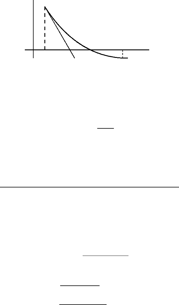
14.2 Newton-Raphson Method

Newton’s method is a widely-used classical method for ﬁnding the solu-

tion to a nonlinear univariate function of f (x) on the interval [a, b]. It

is also referred to as the Newton-Raphson method. At any given point

shown in Fig. 14.1, we can approximate the function by a Taylor

series

f(x

n+1

) = f(x

+ ∆x) ≈ f(x

) + f

)∆x, (14.4)

where

∆x = x

n+1

− x

, (14.5)

which leads to

n+1

− x

= ∆x ≈

f(x

n+1

) − f(x

)

, (14.6)

n+1

≈ x

f(x

n+1

) − f(x

)

. (14.7)

14.2 Newton-Raphson Method 197

f(x)

∗

n+1

Figure 14.1: Newton’s method of approximating the root x

∗

n+1

from the previous value x

Since we try to ﬁnd an approximation to f (x) = 0 with f (x

n+1

), we

can use the approximation f (x

n+1

) ≈ 0 in the above expression. Thus

we have the sta ndard Newton iterative formula

n+1

= x

−

f(x

)

. (14.8)

The iteration procedure starts from an initial guess value x

and co n-

tinues until certain criteria are met. A good initial guess will use fewer

steps; however, if there is no obvious initial good starting point, you

can start at any point on the interval [a, b]. B ut if the initial value is

too far fr om the true zero, the iteration process may fail. So it is a

good idea to limit the number of iterations.

Example 14.2: To ﬁnd the ro ot of

f(x) = x − e

−sin x

= 0,

we use Newton-Raphson method starting from x

= 0. We know that

(x) = 1 + e

−sin x

cos x,

and thus the iteration formula becomes

n+1

= x

−

− e

−sin x

1 + e

−sin x

cos x

Since x

= 1, we have

= 0 −

0 − e

−sin 0

1 + e

−sin 0

cos 0

= 0.5000000000,

= 0.5 −

0.5 − e

−sin 0.5

1 + e

−sin 0.5

cos 0.5

≈ 0.5771952598

198 Chapter 14. Numerical Methods

≈ 0.5787130827, x

≈ 0.5787136435.

We can see that x

(only three iterations) is very close (to the 6th decimal

place) to the true root which is x

∗

≈ 0.57871364351972, while x

accurate to the 10th decimal plac e .

We have seen that Newto n-Raphson’s method is very eﬃcient and

that is why it is so widely used. Using this method, we can virtually

solve almost all root-ﬁnding problems. However, this method is not

applicable to carrying out integration.

14.3 Numerical Integration

For any smooth function, we can always calculate its derivatives by

direct diﬀerentiation; however, integration is often diﬃcult even for

seemingly simple integrals such as the error function

erf(x) =

√

−u

du. (14.9)

The integra tion of this simple integrand exp(−u

) does not lead

to any simple explicit expression, which is why it is often written as

erf(), referred to as the error function. If we pick up a mathematical

handb ook, we know that erf(0) = 0, and erf(∞) = 1, while

erf(0.5) ≈ 0.52049, erf(1) ≈ 0.84270. (1 4.10)

If we want to calculate such integrals , numerical integration is the best

alternative.

Now if we want to numerically evaluate the following integral

I =

f(x)dx, (14 .11)

where a and b are ﬁxed and ﬁnite; we know that the value of the integra l

is exactly the total area under the curve y = f(x) between a and b.

As both the integral and the area can be considered as the sum of

the values over many small intervals, the simplest way of evaluating

such numerical integration is to divide up the integral interval into n

equal small sections and split the area into n thin strips of width h

so that h ≡ ∆x = (b − a)/n, x

= a and x

= ih + a(i = 1, 2, ..., n).

The values of the functions at the dividing points x

are denoted as

= f (x

), and the value at the midpoint between x

and x

i+1

labeled as y

i+1/2

= f

i+1/2

= f(x

i+1/2

) = f

i+1/2

, x

i+1/2

+ x

i+1

. (14.12)

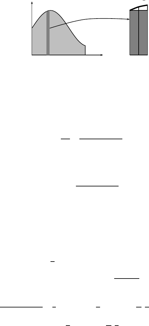
14.3 Numerical Integration 199

f(x)

i+1

Figure 14.2: Integral as a sum of multiple thin stripes.

The accuracy of s uch approximations depends on the number n and

the way to approximate the cur ve in each interval.

Figure 14.2 shows such an interval [x

, x

i+1

] which is exaggerated

in the ﬁgure for clarity. The curve segment between P and Q is ap-

proximated by a straight line with a slope

∆y

∆x

f(x

i+1

) − f(x

)

, (14.13)

which approaches f

i+1/2

) at the midpoint point when h → 0.

The trapezium (formed by P , Q, x

i+1

, and x

) is a better approxi-

mation than the rectangle (P , S, x

i+1

and x

) because the former has

an area

f(x

) + f(x

i+1

)

h, (14.14)

which is closer to the area

i+1

f(x)dx, (14.15)

under the curve in the small interval x

and x

i+1

. If we use the area A

to approximate I

, we have the trapezium rule of numerical integration.

Thus, the integral is s imply the s um of all these small trapeziums, and

we have

I ≈

+ 2(f

+ f

+ ... + f

n−1

) + f

]

= h[f

+ f

+ ... + f

n−1

+ f

)

]. (14.16)

From the Taylor series, we know that

f(x

) + f(x

i+1

)

≈

[f(x

i+1/2

) −

i+1/2

) +

(

)

i+1/2

)]

+[f(x

i+1/2

) +

i+1/2

) +

(

)

i+1/2

)]