Zhu J. Applications of Fourier Transform to Smile Modeling: Theory and Implementation
Подождите немного. Документ загружается.


58 3 Stochastic Volatility Models
3.3.2 Derivation of CFs
Sch
¨
obel and Zhu (1999) applied the expectation approach, as shown in the Heston
model, to derive the analytic solutions for CFs. Readers can verify that the PDE
approach is no longer valid for the stochastic volatility model in (3.28), which is a
evidence that expectation approach is more general for PDE approach. Here we do
not show the derivations in details and give directly the analytic forms of CFs.
f
1
(
φ
)=E
Q
[g
1
(T)exp(i
φ
x(T))] = E
Q
[exp(−rT −x
0
+(1 + i)
φ
x(T))]
= exp
i
φ
(x
0
+ rT) −
ρ
2
σ
(1+i
φ
)v
2
0
−
1
2
(1+i
φ
)
ρσ
T
× E
Q
exp
−s
11
T
0
v
2
(t)dt −s
21
T
0
v(t)dt + s
31
v
2
(T)
= exp
i
φ
(rT + x
0
)
cf
SZ
1
(
φ
) (3.31)
with
cf
SZ
1
(
φ
)=exp
−s
31
v
2
0
−
1
2
(1+i
φ
)
ρσ
T
× E
Q
exp
−s
11
T
0
v
2
(t)dt −s
21
T
0
v(t)dt + s
31
v
2
(T)
.
(3.32)
The parameters s
11
,s
21
,s
31
are defined as follows:
s
11
= −
1
2
(1+i
φ
)((1+i
φ
)(1−
ρ
2
) −1 + 2
ρκσ
−1
),
s
21
=
ρκθ
σ
(1+i
φ
),
s
31
=
ρ
2
σ
(1+i
φ
).
We set
y(v
0
,T)=E
Q
exp
−s
11
T
0
v
2
(t)dt −s
21
T
0
v(t)dt + s
31
v
2
(T)
.
According to the Feynman-Kac theorem, y shall satisfy the following PDE,
∂
y
∂
T
= −(s
21
v
2
+ s
21
v)y +
κ
(
θ
−v)
∂
y
∂
v
+
1
2
σ
2
∂
2
y
∂
v
2
(3.33)
with a boundary condition
y(v
0
,0)=exp(s
31
v
2
0
).

3.3 The Sch
¨
obel-Zhu Model 59
This PDE has the following solution,
y(v
0
,T)=exp
1
2
H
3
(T)v
2
0
+ H
4
(T)v
0
+ H
5
(T)
, (3.34)
where
H
3
(T)=
κ
σ
2
−
γ
1
σ
2
γ
4
(sinh(
γ
1
T)+
γ
2
cosh(
γ
1
T)),
H
4
(T)=
1
γ
1
γ
4
σ
2
× [(
κθγ
1
−
γ
2
γ
3
)(1−cosh(
γ
1
T)) −(
κθγ
1
γ
2
−
γ
3
)sinh(
γ
1
T)],
H
5
(T)=−
1
2
ln(
γ
4
)+
sinh(
γ
1
T)
2
γ
3
1
γ
4
σ
2
[(
κθγ
1
−
γ
2
γ
3
)
2
−
γ
2
3
(1−
γ
2
2
)]
+
γ
3
γ
3
1
γ
4
σ
2
(
κθγ
1
−
γ
2
γ
3
)(
γ
4
−1)+
T
2
γ
2
1
σ
2
[
κγ
2
1
(
σ
2
−
κθ
2
)+
γ
2
3
]
with
γ
1
=
2
σ
2
s
11
+
κ
2
,
γ
2
=
κ
2
θ
−s
21
σ
2
,
γ
3
=
1
γ
1
(
κ
−2
σ
2
s
31
),
γ
4
= cosh(
γ
1
T)+
γ
2
sinh(
γ
1
T).
The second CF f
2
(
φ
) has a similar solution to f
1
(
φ
) and takes the following
form,
f
2
(
φ
)=E
Q
[g
1
(T)exp(i
φ
x(T))] = E
Q
[exp(−rT −x
0
+(1 + i)
φ
x(T))]
= exp
i
φ
(x
0
+ rT) −
ρ
2
σ
i
φ
v
2
0
−
1
2
i
φρσ
T
× E
Q
exp
−s
12
T
0
v
2
(t)dt −s
22
T
0
v(t)dt + s
32
v
2
(T)
= exp
i
φ
(rT + x
0
)
cf
SZ
2
(
φ
) (3.35)
with
cf
SZ
2
(
φ
)=exp
−s
32
v
2
0
−
1
2
i
φρσ
T
× E
Q
exp
−s
12
T
0
v
2
(t)dt −s
22
T
0
v(t)dt + s
32
v
2
(T)
,
(3.36)
where s
12
,s
22
,s
32
take the following forms,

60 3 Stochastic Volatility Models
s
12
= −
1
2
i
φ
(i
φ
(1−
ρ
2
) −1 + 2
ρκσ
−1
),
s
22
=
ρκθ
σ
i
φ
,
s
32
=
ρ
2
σ
i
φ
.
In order to compute f
2
(
φ
), s
k1
in
γ
j
, j = 1, 2, 3, 4, should be replaced by s
k2
corre-
spondingly.
3.3.3 Numerical Examples
Here we give some numerical examples to demonstrate the properties of Sch
¨
obel-
Zhu model. For comparison, we shall choose the suitable Black-Scholes (BS) option
prices as benchmark. The first possible benchmark is the BS price using the expected
average variance AV as input. As shown in Ball and Roma (1994), if v(t) follows a
mean-reverting Ornstein-Uhlenbeck process, we can calculate AV as follows:
AV =
σ
2
2
κ
+
θ
2
+
1
T
2
θ
(v
0
−
θ
)
κ
(1−e
−
κ
T
) −
σ
2
−2
κ
(v
0
−
θ
)
2
4
κ
2
(1−e
−2
κ
T
)
.
(3.37)
We denote the BS prices evaluated in this manner by BS
1
. The second alterna-
tive as in Stein and Stein is to calculate the BS option prices according to the spot
volatility v(t) with
κ
,
ρ
and
σ
as nil. This calculated BS prices labeled to BS
2
are
identical to these prices by using the BS formula with a constant volatility v(t) be-
ing equal to
θ
. Heston (1993) used the BS prices with a volatility which equates
the square root of variance of the spot stock returns up to maturity. His benchmark
is then dependent on the correlation
ρ
and makes comparisons remarkably com-
plicated.
6
It is difficult to say which benchmark is better. Evaluating BS
1
has an
implication that volatility follows a stochastic process and is not constant. This is
in contradiction with the BS’s assumption. In this sense, BS
1
is not a logically con-
sistent but only ad hoc BS value. In contrast, BS
2
implies that the volatility keeps
constant and equates the initial value v
0
. Therefore, both BS
1
and BS
2
might (not) be
a right benchmark for comparison with the exact option prices. However, as shown
by numerical examples, both benchmarks do not distinguishes each other remark-
ably.
6
Since Heston’s BS benchmark is a function of the correlation
ρ
, every model option value has a
corresponding Heston’s benchmark. Thus, we will lose some clarity in comparison if using Hes-
ton’s benchmark although it is reasonable in some senses.
3.3 The Sch
¨
obel-Zhu Model 61
In Table (3.2), we choose the parameters suggested by Stein and Stein. In order
to show the impact of correlation on the option prices, let
ρ
range from -1.0 to 1.0.
Some observations are in order.
First of all, options with different moneyness have different sensitivity to the cor-
relation
ρ
. The values of at-the-money (ATM) options do not change remarkably
overall. However, the sensitivity of out-of-the-money (OTM) options to
ρ
is more
conspicuous than of in-the-money (ITM) options. For example, in Panel C the rela-
tive changes of the OTM option prices due to the correlation
ρ
for K = 120 is about
±14% of the Stein and Stein value which is here 2.635.
Secondly, a comparison of Panels A, B and C shows that the mean-reversion level
θ
is important for the pricing of options. Keeping other parameters unchanged, the
differential (
θ
−v) (mean-reversion level minus current volatility) has a great impact
on the option values. From Panel A to C, (
θ
−v) is 0, -0.1 and 0.1 respectively,
and the differences in option prices across these panels are mostly between 0.60$
and 1.50$. Since the expectation of the future spot price volatility approaches
θ
, the
prices of options, especially the options with a long-term maturity, should be mainly
affected by
θ
.
Thirdly, as expected, we find the price differences between BS
1
and the model
values with
ρ
= 0 are smallest for all panels. This confirms Ball and Roma’s find-
ing. The good fit of these two values is not surprising since BS
1
is by nature an
approximation for the exact option value with
ρ
= 0. Panel D in Table 2.3 presents
all BS
1
values corresponding to Panels E-G. We can see that the BS
1
values in Panel
D agree very well with the option values in Panel F. However, if
ρ
= 0, the price
bias between BS
1
values and the exact option values are significant. Thus, BS
1
is
not a suitable approximation for the correlation case. It is also not surprising that
the BS
2
values match our model values closely for Panel A where
θ
= v. Stein and
Stein report an overall overvaluation relative to BS
2
due to stochastic volatility. This
upward pricing bias should be caused by the zero correlation assumption between
volatility and its underlying asset returns in Stein and Stein. For
ρ
= 0 the direction
of the movement of S(t) is not affected by stochastic volatility, and any stochas-
tic volatility raises only the additional uncertainty of S(t). Consequently, Stein and
Stein and BS
1
values are greater than BS
2
values in Panel A.
Finally, ITM options and OTM options react to correlation just oppositely.
Whereas ITM options (K = 90,95) decrease in value with increasing correlation
ρ
,
OTM option prices (K = 105,110,115,120) go up. This finding is consistent with
Hull’s (1997, pages 492-500) excellent intuitive explanation of how correlation af-
fects option prices. It is also empirically evident that stock returns are inversely
correlated with the underlying volatilities. Panels A to C show that a negative cor-
relation
ρ
leads to ITM (OTM) option prices in our model that are greater (less)
than the corresponding BS option prices. This feature caused by negative correla-
tion is useful for explaining volatility sneers. The smile pattern is most of the time
not so obvious and appears to be more of a sneer. The monotonic downward slop-
ing of the implied volatility with moneyness displayed in a sneer implies that the
market ITM (OTM) options are undervalued (overvalued) by the BS formula. This
pattern of pricing biases in the BS formula is reported by a number of empirical
62 3 Stochastic Volatility Models
studies as in Nandi (1998), Heston and Nandi (1997), BCC (1997) and MacBeth
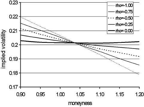
and Merville (1979). Figure (3.1) shows the calibrated implied volatilities in Panel
A where the downward sloping of implied volatility for
ρ
< 0 is significant. The
good fit of our calibrated examples to the empirical picture supports that incorporat-
ing correlation between stock returns and volatilities is a promising way to improve
the performance of option pricing. BCC (1997) and Nandi (1998) reported that tak-
ing stochastic volatility into account is of first-order importance in eliminating the
volatility inconsistence and leads to significant improvements in hedging perfor-
mance, but only in the presence of non-zero correlation. Their results should also be
valid for our model.
In Table (3.3), we examine how the option prices vary with the mean-reverting
level
θ
. The finding that option prices are very sensible to
θ
is confirmed. Since
θ
indicates the long-term level of volatility, this sensitivity can be considered as the
sensitivity of option prices to their volatilities in the long run. Furthermore, it seems
to be that
θ
is more important than the spot volatility v(t) for the pricing of options in
the framework of a mean-reverting process. If the true process of volatility performs
mean-reversion, and option prices are evaluated using the BS formula regardless
of BS
1
or BS
2
, a significant pricing bias will occur although the magnitude of the
pricing bias for BS
1
is smaller than that for BS
2
. All prices in Panel F correspond
to the case of Stein and Stein. The numbers in the first row in panels D, E, F and
G are option prices under the restricted Heston model in the sense of equations
(3.5) and (3.6). The implied zero level of the mean-reversion leads to an overall
undervaluation of options compared with BS
2
.
Table (3.4) demonstrates the impact of
ρ
on Delta
Δ
S
whichisoffirst-order
importance for hedging purposes whenever stochastic volatility models are used.
Firstly, for the given parameters almost all of the Deltas are decreasing with corre-
lation
ρ
except for a few deep-ITM and deep-OTM options across the three Panels
H, I and J. Secondly, the changes of values of near-ATM options relative to the cor-
relation
ρ
are more sensitive than these of deep-ITM and deep-OTM options. The
differences between
Δ
S
in the Sch
¨
obel-Zhu model and the BS model (BS
1
and BS
2
)
for near-ATM options should not be neglected. For a negative correlation, using
Δ
S
of the BS formula and the Stein and Stein model seems to cause a severe under-
hedging for near-ATM options and some OTM options. Furthermore, the long-term
level of volatility
θ
is also important for hedging. Keeping other parameters un-
changed, the greater
θ
is, the smaller (greater)
Δ
S
will be for ITM (OTM) options.
The sensitivity of
Δ
S
to
θ
is remarkable and can be studied more detailed by the
second derivative
Δ
S
θ
. We conclude that an unbiased estimate of
θ
is crucial for
Delta-hedging.
Stochastic volatility models provide us with new insights into derivative security
markets. In this section, we have derived a closed-form pricing formula for the gen-
eral case where volatility is allowed to display arbitrary correlation with the underly-
ing stock price. In comparison with the Heston model, this specification for volatil-
ity performs additional favorite properties such as a direct link to volatility instead
of variance, easy estimation of parameters in a Gaussian framework. As discussed
earlier, the negligibly small possibilities for negative volatilities in such a process
3.4 Double Square Root Model 63
do not raise a serious problem in option pricing. Additionally, since in a diffusion
context negative volatilities only mean that upward moves of the driving Brownian
motion become downward moves of the stock price and vice versa, we believe that
this is not a severe theoretical restriction and suggest this new closed-form pricing
formula as an alternative to Heston’s solution: Not surprisingly, squared volatilities
never become negative here either.
Fig. 3.1 Model volatility smile for negative and zero correlation, calculated from Panel A
in Table (3.2)
3.4 Double Square Root Model
3.4.1 Model Setup and Properties
In this section, we consider a new variant of stochastic volatility model where
squared volatility is specified as a double square root process. This is a process that
was originally introduced by Longstaff (1989) to model stochastic interest rates,
in order to explain non-linear term structure observed in yield curves. Longstaff
showed that the non-linear model driven by double square root process outperforms
the CIR model driven by square root process for the 1964-1986 period in explain-
ing the behavior of yield curves. Since stochastic variance and stochastic interest
rates share many same characteristics, it is interesting to adopt mean-reverting dou-
ble square root to model the dynamics of stochastic variances V(t). Heston (1993)
considered also the stochastic volatility model with double square root process in

64 3 Stochastic Volatility Models
ρ
K
90 95 100 105 110 115 120
BS
2
15.118 11.342 8.142 5.584 3.658 2.293 1.377
BS
1
15.152 11.391 8.203 5.650 3.722 2.349 1.422
-1.00 15.416 11.617 8.307 5.576 3.468 1.966 0.995
-0.75 15.355 11.562 8.275 5.585 3.525 2.063 1.110
-0.50 15.292 11.503 8.243 5.595 3.582 2.156 1.218
-0.25 15.225 11.443 8.210 5.606 3.638 2.246 1.321
0.00 15.155* 11.379* 8.176* 5.617* 3.694* 2.333* 1.420*
0.25 15.081 11.313 8.141 5.628 3.749 2.416 1.514
0.50 15.003 11.243 8.106 5.640 3.803 2.497 1.605
0.75 14.919 11.169 8.070 5.652 3.856 2.576 1.693
1.00 14.828 11.092 8.034 5.665 3.909 2.653 1.777
A:
θ
= 0.2,
κ
= 4,
σ
= 0.1,v = 0.2, T = 0.5,S = 100,r = 0.0953
ρ
K
90 95 100 105 110 115 120
BS
1
14.501 10.348 6.829 4.132 2.282 1.150 0.530
-1.00 14.730 10.600 6.976 4.057 1.977 0.739 0.179
-0.75 14.679 10.541 6.936 4.066 2.051 0.853 0.279
-0.50 14.626 10.480 6.894 4.075 2.121 0.957 0.371
-0.25 14.572 10.415 6.849 4.085 2.189 1.053 0.458
0.00 14.515* 10.346* 6.803* 4.093* 2.254* 1.144* 0.542*
0.25 14.456 10.271 6.753 4.102 2.316 1.230 0.621
0.50 14.495 10.191 6.701 4.110 2.376 1.311 0.698
0.75 14.330 10.103 6.645 4.117 2.433 1.389 0.773
1.00 14.261 10.005 6.587 4.125 2.489 1.463 0.845
B:
θ
= 0.1,
κ
= 4,
σ
= 0.1,v = 0.2, T = 0.5,S = 100,r = 0.0953
ρ
K
90 95 100 105 110 115 120
BS
1
16.111 12.666 9.711 7.264 5.305 3.786 2.646
-1.00 16.357 12.846 9.777 7.186 5.084 3.449 2.235
-0.75 16.298 12.800 9.755 7.198 5.133 3.531 2.340
-0.50 16.236 12.751 9.732 7.210 5.182 3.611 2.441
-0.25 16.172 12.702 9.710 7.223 5.230 3.690 2.540
0.00 16.106* 12.651* 9.687* 7.237* 5.279* 3.768* 2.635*
0.25 16.037 12.598 9.665 7.251 5.328 3.844 2.728
0.50 15.964 12.544 9.642 7.265 5.377 3.919 2.819
0.75 15.889 12.489 9.620 7.280 5.426 3.993 2.908
1.00 15.810 12.432 9.598 7.296 5.475 4.065 2.994
C:
θ
= 0.3,
κ
= 4,
σ
= 0.1,v = 0.2, T = 0.5,S = 100,r = 0.0953
The numbers with * correspond to the model of Stein and Stein.
Table 3.2 The impact of the correlation
ρ
on option prices. The prices of ITM calls (OTM calls)
decrease (increase) with increasing correlations
ρ
.
his appendix, but did not give an explicit solution for options. Following the method
in his paper, i.e., the PDE approach, we find that it leads to a rather cumbersome
procedure and can not decompose the PDEs into several ordinary differential equa-
tions which can be solved successively. Here we will give an explicit solution by
applying stochastic calculus.
In fact, the generator of a double square root process is a Brownian motion with
drift. To see this, we assume that volatility v(t) is governed by the following process,

3.4 Double Square Root Model 65
θ
K
90 95 100 105 110 115 120
BS
2
14.515 10.374 6.867 4.175 2.322 1.180 0.550
0.0 14.194* 9.510* 5.277* 2.213* 0.654* 0.132* 0.018*
0.1 14.333 9.990 6.282 3.499 1.708 0.728 0.272
0.2 14.864 10.962 7.662 5.060 3.155 1.859 1.037
0.3 15.757 12.213 9.187 6.707 4.755 3.278 2.200
D: The BS
1
values using the expected average volatility as input
κ
= 4,
σ
= 0.1,v = 0.15, T = 0.5,S = 100,r = 0.0953
θ
K
90 95 100 105 110 115 120
0.0 14.189* 9.459* 5.141* 2.173* 0.763* 0.244* 0.075*
0.1 14.262 9.842 6.132 3.466 1.812 0.895 0.425
0.2 14.723 10.804 7.551 5.044 3.239 2.014 1.220
0.3 15.608 12.082 9.109 6.703 4.828 3.414 2.376
E:
ρ
= 0.5,
κ
= 4,
σ
= 0.1,v = 0.15, T = 0.5,S = 100,r = 0.0953
θ
K
90 95 100 105 110 115 120
0.0 14.200* 9.527* 5.267* 2.170* 0.645* 0.150* 0.030*
0.1 14.351 9,997 6.254 3.451 1.679 0.731 0.292
0.2 14.871 10.952 7.632 5.022 2.124 1.845 1.040
0.3 15.754 12.198 9.161 6.676 4.727 3.259 2.192
F:
ρ
= 0.0,
κ
= 4,
σ
= 0.1,v = 0.15, T = 0.5,S = 100,r = 0.0953
θ
K
90 95 100 105 110 115 120
0.0 14.225* 9.600* 5.372* 2.152* 0.504* 0.061* 0.004*
0.1 14.441 10.130 6.361 3.435 1.529 0.545 0.155
0.2 15.003 11.084 7.710 5.003 3.004 1.660 0.842
0.3 15.887 12.306 9.213 6.652 4.626 3.097 1.995
G:
ρ
= −0.5,
κ
= 4,
σ
= 0.1,v = 0.15, T = 0.5,S = 100,r = 0.0953
The numbers with * correspond to the restricted Heston model.
Table 3.3 The impact of the mean level
θ
on option prices. Option prices increase with increasing
mean levels
θ
.
dv(t)=
μ
dt +
ε
dW
2
(t),
where
μ
and
ε
are constant, and dW
1
dW
2
=
ρ
dt. Applying It
ˆ
o’s lemma yields the
dynamics of the variances,
dv
2
(t)=[
ε
2
+ 2
μ
v(t)]dt + 2
ε
v(t)dW
2
(t)
=
κ
[
θ
−v(t)]dt +
σ
v(t)dW
2
(t)
with
κ
= −2
μ
,
κθ
=
ε
2
,
σ
= 2
ε
.
Now let V(t)=v
2
(t) denote the squared volatility, we then arrive at a process for
instantaneous variances V(t) as follows:
dV(t)=
κ
θ
−
V(t)
dt +
σ
V(t)dW
2
(t). (3.38)
Since two square root terms arise in this process, it is thus referred to as double
square root process. The necessary condition for generating process (3.38)isthe

66 3 Stochastic Volatility Models
ρ
K
90 95 100 105 110 115 120
BS
2
0.8755 0.7795 0.6582 0.5249 0.3950 0.2807 0.1890
BS
1
0.8731 0.7773 0.6571 0.5253 0.3968 0.2836 0.1922
-1.00 0.8751 0.7949 0.6895 0.5644 0.4299 0.3002 0.1883
-0.75 0.8708 0.7916 0.6825 0.5547 0.4204 0.2941 0.1881
-0.50 0.8751 0.7881 0.6751 0.5449 0.4113 0.2889 0.1883
-0.25 0.8752 0.7844 0.6673 0.5350 0.4027 0.2843 0.1887
0.00 0.8754* 0.7802* 0.6591* 0.5251* 0.3945* 0.2802* 0.1891*
0.25 0.8756 0.7757 0.6504 0.5153 0.3868 0.2765 0.1896
0.50 0.8759 0.7707 0.6413 0.5055 0.3795 0.2732 0.1899
0.75 0.8761 0.7649 0.6317 0.4957 0.3725 0.2701 0.1904
1.00 0.8761 0.7584 0.6216 0.4862 0.3659 0.2673 0.1907
H:
θ
= 0.2,
κ
= 4,
σ
= 0.1,v = 0.2, T = 0.5,S = 100,r = 0.0953
ρ
K
90 95 100 105 110 115 120
BS
1
0.9344 0.8401 0.6937 0.5166 0.3440 0.2047 0.1093
-1.00 0.9246 0.8490 0.7302 0.5684 0.3816 0.2048 0.0763
-0.75 0.9267 0.8479 0.7229 0.5554 0.3694 0.2025 0.0867
-0.50 0.9293 0.8467 0.7151 0.5424 0.3584 0.2012 0.0947
-0.25 0.9323 0.8456 0.7068 0.5293 0.3485 0.2003 0.1012
0.00 0.9359* 0.8445* 0.6978* 0.5163* 0.3395* 0.1996* 0.1065*
0.25 0.9403 0.8433 0.6881 0.5033 0.3311 0.1989 0.1111
0.50 0.9458 0.8421 0.6774 0.4903 0.3234 0.1982 0.1149
0.75 0.9530 0.8404 0.6656 0.4773 0.3163 0.1975 0.1182
1.00 0.9629 0.8379 0.6526 0.4645 0.3095 0.1967 0.1211
I:
θ
= 0.1,
κ
= 4,
σ
= 0.1,v = 0.2, T = 0.5,S = 100, r = 0.0953
ρ
K
90 95 100 105 110 115 120
BS
1
0.8225 0.7358 0.6373 0.5341 0.4334 0.3410 0.2606
-1.00 0.8317 0.7552 0.6646 0.5644 0.4606 0.3599 0.2682
-0.75 0.8300 0.7512 0.6584 0.5568 0.4532 0.3541 0.2652
-0.50 0.8282 0.7469 0.6519 0.5492 0.4459 0.3487 0.2626
-0.25 0.8264 0.7424 0.6452 0.5416 0.4389 0.3437 0.2604
0.00 0.8243* 0.7376* 0.6383* 0.5339* 0.4322* 0.3390* 0.2584*
0.25 0.8221 0.7324 0.6311 0.5263 0.4256 0.3347 0.2566
0.50 0.8196 0.7269 0.6237 0.5187 0.4193 0.3306 0.2550
0.75 0.8169 0.7210 0.6162 0.5112 0.4133 0.3267 0.2536
1.00 0.8137 0.7147 0.6084 0.5038 0.4074 0.3231 0.2522
J:
θ
= 0.3,
κ
= 4,
σ
= 0.1,v = 0.2, T = 0.5,S = 100,r = 0.0953
The numbers with * correspond to the model of Stein and Stein.
Table 3.4 The impact of the correlation
ρ
on Delta
Δ
S
. Deltas decrease with increasing correlations
ρ
only for near-ATM options.
restriction
σ
2
= 4
κθ
with which some special expected values of V(t) can be cal-
culated analytically. Additionally, zero may be an accessible boundary under this
restriction.
7
Generally, we have two ways to adjust the above double square root process
to a risk-neutral process by market price of risk. More precisely, one approach is
7
When 0 <
σ
2
<
κθ
, zero value of v(t) is inaccessible and no boundary condition can be imposed
at zero. When 0 <
κθ
<
σ
2
, zero is accessible. See Longstaff (1989).

3.4 Double Square Root Model 67
to introduce a market price of volatility risk, the other is to utilize a market price
of variance risk. By the first approach, the market price of risk is equal to
λ
(t)=
λ
v(t)=
λ
V(t), which implies a risk-neutral process as follows:
dV(t)=
κθ
−(
κ
−
λ
)
V(t)
dt +
σ
V(t)dW
2
(t)
=
κ
∗
θ
∗
−
V(t)
+
σ
V(t)dW
2
(t) (3.39)
with
κ
∗
=
κ
−
λ
and
θ
∗
=
κθ
/
κ
∗
. Hence, the obtained risk-neutral process keeps
the same structure as its original counterpart. In the second approach, we introduce
an identical market price of risk as in the Heston model, i.e.,
λ
(t)=
λ
V(t).This
interpretation of market price of risk
λ
leads to the following risk-neutral process,
dV(t)=
κθ
−
κ
V(t) −
λ
V(t)
dt +
σ
V(t)dW
2
(t)
=
1
4
σ
2
−
κ
V(t) −
λ
V(t)
dt +
σ
V(t)dW
2
(t), (3.40)
which has a mixed structure of double and single square root processes. Note the
risk-neutral process of first approach is a special case of the one of second approach,
we discuss the second approach for generality. By setting
λ
= 0, the price formula
given below is reduced to the price formula with market price of volatility risk.
Compared with the single square root process (3.4) in the Heston model, the dou-
ble square root process has some distinct features. Firstly, the mean level of variance
here does not take an unambiguous value since the constant
1
4
σ
2
measures the long
term level of
κ
V(t)+
λ
V(t). This mixed structure of the drift provides us with
a weighted value of volatility and variance as mean level. Due to the restriction
σ
2
= 4
κθ
, it seems that
1
4
σ
2
as long term value of (
κ
V(t)+
λ
V(t)) is small in
many cases. For example, for
σ
= 0.5 and V
0
= 0.2, the reasonable values of
κ
should not be larger than 1. This means that volatility shocks to stock price process
are rather persistent and revert to mean level very slowly. Another feature of this
model is that, as mentioned above, the generating process of double square root dy-
namics is a Brownian motion with drift and therefore is not stationary, and volatility
itself does not perform mean-reversion, hence such specifications of volatility and
variance are not tenable from aprioritheoretical consideration. On the other hand,
we have one parameter less to estimate empirically because of the above parameter
restriction. Numerical examples show that this stochastic volatility model can still
capture most essential features of volatility smile.
The double square process will be identical to single square process if we set
some special parameter values,
κ
DSR
= 0,
θ
SR
= 0,
κ
SR
=
λ
DSR
,
where the subscripts DSR and SR stand for double square root process and square
root process respectively. Obviously, such parameter values are not realistic.
It is not hard to obtain the following two CFs for the double square root process: