Werner Leonhard Control of Electrical Drives

41

,

III

3.

Integration

or

the

Simplified

Equation

or

Motion

:Ci

(V

+

1)

~

Xi(V)

+ F['Pi(V),

'Pi(V

- 1),

...

] ,

(3.27)

w!ln"!! F is a linear combination

of

the

functions

'Pi

at

previous intervals.

'I '

It

ere exists a large

number

of

integration

formulae which differ

in

complex-

il

,y, i.e.

computing

time, sensitivity to numerical

instability

and

accuracy [22].

'l'

lte

ones

best

known

are

square-, trapezoidal-

and

Simpsons-rules, further-

IIl<lr

e

the

Newton-

and

Runge-Kutta-algorithms.

Because

of

its favourable

propertí

es

the

last mentioned

algorithm

is widely usedj

it

is usually avail-

:th\e as a complete

subroutine

so

that

only

the

functions

'Pi

and

the

initial

CO

llditions

Xi(O)

need

to

be inserted as well as

the

integration

interval

Llt

;\,

11<1

the

time

t

2

at

which

the

integration

is

to

be

terminated.

Often

the

in-

Lq

,;ration interval Llt is chosen automatically, depending

on

the

functions

(Pi a

nd

a specified accuracy limito We

are

not

going

to

discuss details of

IIll1nerical integrationj

there

can

be

subtle

problems

interrelating

step

size,

<t.c

cnracy

and

numerical stability. Since a large

number

of

steps

may

have

Lo

he

computed

sequentially, even

minute

systematic

errors

can

accumulate

IIl1d

er unfavourable conditions.

Obvíously

the

two differential equations, Eqs. (2.1), (2.2), correspond

to

I.his

general schemej when

taking

the

angle

of

rotation

into account,

the

order is n =

2,

i.

e.

a very small system

of

differential equations results.

The

,~

Lat

e

v

ar

iables

are

the

rotational

01' linear speed

and

the

angle

of

rotation

or

I.Iw

liJl

ea

r distance.

These

variables represent

storage

effects and, hence,

are

C()lItiJlllOUS.

If

a more

accurate

description is desired,

the

electrical

transients

!Iav

(! to

be

included,

thus

increasing the

number

of

differential

equations

and

sl"d,

(!

variablesj this is discussed in

later

sections.

Wlwll a

tímetable

for a

branch

of

a railway is

to

be computed,

it

is neces-

l:a

l'y 1,0

take

into account

the

mass M

of

the

trains

, including

the

equivalent

ill('rlú

01'

the

wheel sets,

the

speed-dependent

driving forces

of

the

loco-

II

II,

Li

v(!s,

dista

nce-dependent

conditions, such as grades, curves

or

speed re-

Il

l.ricl.io!l

s, as well as

maximum

values for deceleration.

The

task

requires

the

:;i

111111

tancous solutíon

of

the

differential equations for velo city

and

distance

dv

1

-1

--

= M

[JM(V,

t) -

h(s,

v, t)] ,

( t

ds

dt =

V,

wll(!l'('

1M

is

the

internal

driving force of

the

locomotive

and

h is

the

to-

tal

loar!

force, íncluding frictional

and

braking

forces

a.s

well as

gravitational

l'ol'('

cs

Oll

grades.

The

task

of

finding an acceptaiJl('

tillldable

is

an

optimisa-

I,

i(lll

prohlc

lJI

of

cO

Ilside

rable

complexity, sinc(' lIlally cOllstraiJlts

and

bound-

:

lr

,Y

cOlldi(

,

ioIl

S

llIu

st

h(

! tõlken into

aCCOllnl..

'l'llú; indlld,':;

Lhe

Il

S(!

of

th

e

same

Lr:lt'k

I,y

I.r:tills Itavillg diffcrcllt I\.('cdcra(.ioll

:1

,

lId

vl'lociLy

lilllÍts, such

a.'i

in-

L('IT

,

iLy

<lI'

II(

!il

VY

I

~

o()d

:;

(,

nlÍIIH

.

Th

e

pro!'I"11I

(

'!l

1I

lillly

IIl'

Holv"d

I,

y itmatioll,

...

·p(

·

II.1.(

·

(lIy

iIlL(

·I'

,I'II

,l.illl',I':qH. (2

.1)

,

('

.l.'2

)

wi1.1t

dl

ll'(

'I'I·lIl. llIl

l.i

lll (·

(lIldil.i(lII

K. 'J'oday

1.1

11

1:

1II

t.

,y

piC'

l\.

1

1'1,,1,),

'

111

r"

"

11I111I(

'rk

ld 1

III."

I'

,

I'

/

tI

,ll lI' w

ll

,

1t

I

I,

dil',

d,1I1

(IIHlplll,(·

r.

IIl1

wl'v

\'I . I

II

1.11

,'

1"

1'11

,

11

, I

lI

ld

1.11

I"

,

~iI

,lv,·

,

d

Cl

ll

llil

l/

tll

y

lI

i.

I"I',

1·

.!"I

.1.1<

ItI

1111'111,,,11:.

3.3 Numerical

and

Graphical

Integration

Since

it

cannot

be ruled

out

that,

even today,

this

may have

to

be

done

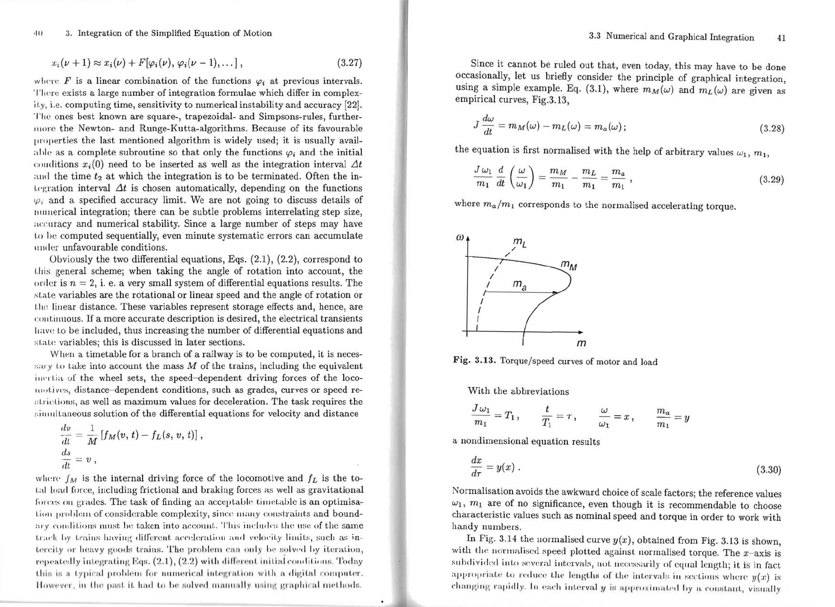
occasionally, let us briefly consider

the

principIe

of

graphical

integration,

using a simple example. Eq. (3.1), where mM(w)

and

mdw)

are

given as

empirical curves,

Fig

.3.13,

dw

J

di

=

mM(w)

-

mdw)

=

ma(w);

(3.28)

the

equation

is first normalised

with

the

help

of

arbitrary

values

WI,

mI,

J

WI

~

(~)

_

mM

_ mL _

ma

(3

.29)

mI

dt

WI

-

mI mI

-

mI

'

where

ma/mI

corresponds to

the

normalised accelerating torque.

cu

mL

/

m

Fig.

3.13.

Torque/speed

curves

or

motor

and

load

With

the

abbreviations

JWI

=

TI,

t

ma

-T=r

W =

X,

mI

=y

1 '

WI

a nondimensional

equation

results

dx

dr

=y(x).

(3.30)

Normalisation

avoids

the

awkward choice

of

scale factors;

the

reference values

WI,

mI

are

of

no significance, even

though

it

is recommendable

to

choose

characteristic

values such as

nominal

speed

and

torque

in

order

to

work with

handy

numbers

.

ln

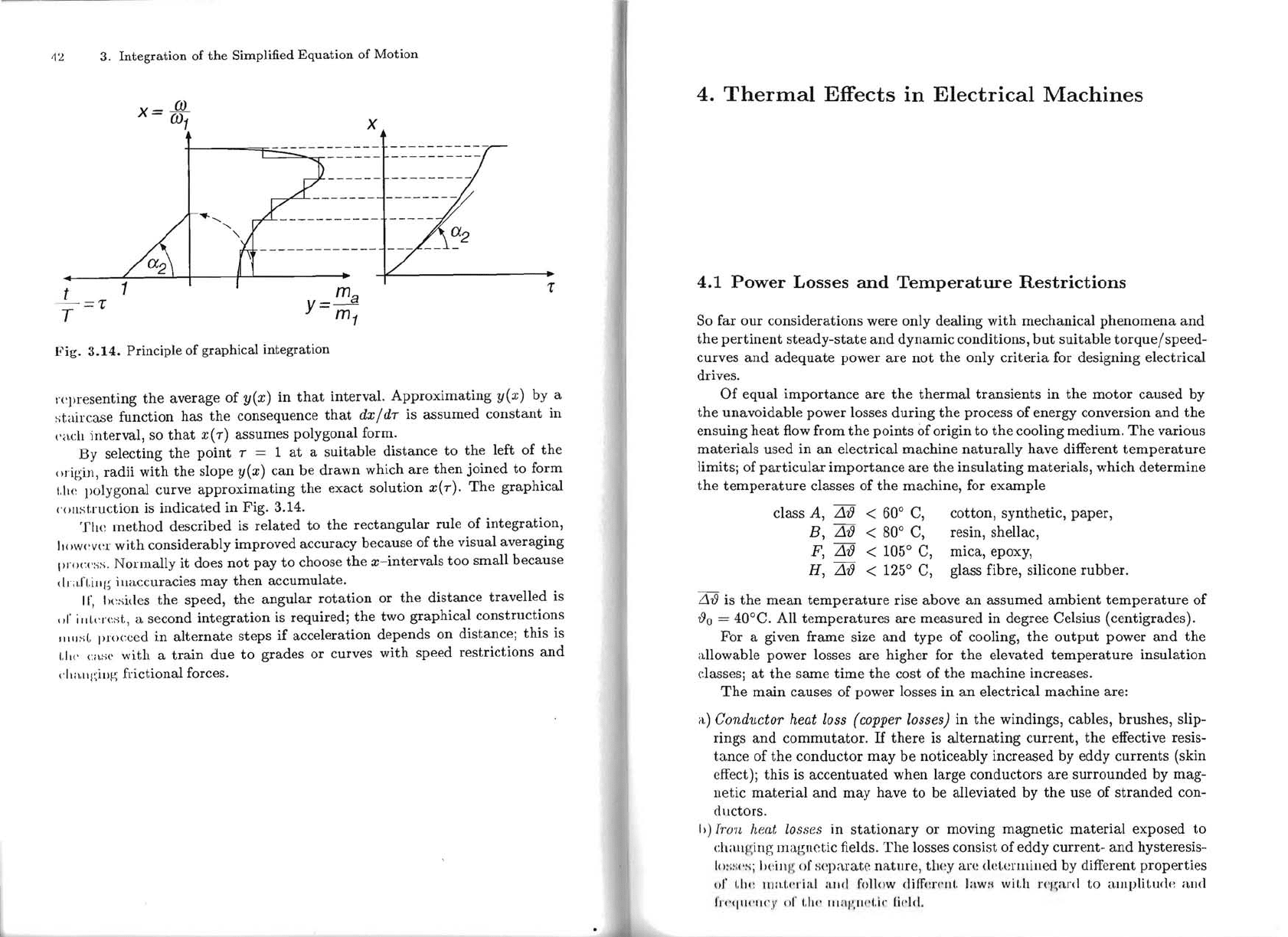
Fig. 3.14

the

normalised curve

y(x),

obtained

from Fig. 3.13 is shown,

with

t.lt

p

lI

ol:llIn

lif

;cd speed

plotted

against Ilormalised torque.

The

x- axis

is

sllbdividcd

illl.o

scv(

~

r;tl

illt(!l'vals,

JlOt,

!)(!cPHsarily

of

c<.J.

l1al

lcn

gt

h; it is in fact

:l.pPl'Opri:i.I

,,'

1.0

/'C'dll('"

1,

111'

1(

!

lIgLhH

01'

1.

I

li'

illkrv:d:;

iII

/;

cdiolJS wheJ'c

y(:,

:) iH

('Ia

ii

"1',1

" I',

I'

lI.

lIidl

y,

111":,,1'11

illl.(·rV:I

,1 y

i:

: ' i.J'I"'

II

'

"II

:

tf

,

(·cJ

h,Y

II,

(·IIII

I<II.

il.III.

,

vl

!i

ll

a

lly

I\~

3.

Integration

of

the

Simplified

Equation

of

Motion

01

x=

01

1

x

-----..........

.......

ma

y=

m

1

t 1

r

T

=r

Fig.

3.14.

PrincipIe

of

graphical

integration

rCJlr

esenting

the

average of y(x) in

that

interval. Approximating y(x) by a

~it.airc

as

e

function has

the

consequence

that

dx

j

dr

is assumed

constant

in

('<l.c!t

interval, so

that

x( r) assumes polygonal

formo

By selecting

the

point

r = 1

at

a suitable distance

to

the

left of

the

origin,

radii with

the

slope y(x)

can

be drawn which are

then

joined to form

Lhe

Jlolygonal curve

approximating

the

exact solution x( r).

The

graphical

(,()Ilst

,ruction is indicated in Fig. 3.14.

Tlt

e

method

described is related

to

the

rectangular

rule of integration,

"Ow(

'

v(

~

r

with

considerably improved accuracy because of

the

visual averaging

pro

('.

('

:.;s.

Normally

it

does

not

pay

to

choose

the

x-intervals

too

small because

dri

lJl.illg

illaccuracies may

then

accumulate.

I

r,

I

)(

~s

i<l

e

s

the speed,

the

angular

rotation

or

the

distance travelled is

"r

iril

,

('r<

:s

t, a second

integration

is required;

the

two graphical constructions

rlllr~il

procced in

alternate

steps if acceleration depends on distance; this

is

1.11<'

<:il

,s

e with a

train

due

to

grades or curves with speed restrictions

and

cltil,lI

g

ill

g frictional forces.

4.

Thermal

Effects

in

Electrical

Machines

4.1

Power

Losses

and

Temperature

Restrictions

80 far

our

considerations were only dealing with mechanical

phenomena

and

the

pertinent

steady-state

and

dynamic conditions,

but

suitable

torquejspeed-

curves

and

adequate

power

are

not

the

only

criteria

for designing electrical

drives.

Of

equal

importance

are

the

thermal

transients

in

the

motor

caused by

the

unavoidable power losses during

the

process of energy conversion

and

the

ensuing

heat

flow from

the

points of origin

to

the

cooling medium.

The

various

materiais used in

an

electrical machine

naturally

have different

temperature

limits; of

particular

importance

are

the

insulating materiais, which determine

the

temperature

classes of

the

machine, for example

class

A,

Lh9

< 60° C,

cotton, synthetic,

paper,

B,

Lh9

< 80° C,

resin, shellac,

F,

Lh9

< 105° C,

mica, epoxy,

H,

Lh9

< 125° C,

glass fibre, silicone rubber.

..119

is

the

mean

temperature

rise above

an

assumed ambient

temperature

of

19

0

= 40°C. All

temperatures

are measured in degree Celsius (centigrades).

For a given frame size

and

type

of cooling,

the

output

power

and

the

allowable power losses

are

higher for

the

elevated

temperature

insulation

classes;

at

the

sarne

time

the

cost of

the

machine increases.

The

main

causes of power losses in

an

electrical machine are:

a)

Conductor

heat loss (copper losses) in

the

windings, cables, brushes, slip-

rings

and

commutator.

If

there

is

alternating

current,

the

effective resis-

tance

of

the

conductor

may

be noticeably increased by eddy

currents

(skin

e

fFect);

this

is

accentuated

when large conductors

are

surrounded by mag-

netic

material

and

may have

to

be alleviated by

the

use of

stranded

con-

ductors.

h) Irou heat losses in

stationary

or moving magnetic

material

exposed

to

dl<tll

ging mar;nctic fields.

The

losses consist of eddy current-

and

hysteresis-

I()

~~;

('s;

IwiJl

I

~

of

separat.c natllfe, tlH!y are

<i(~L

e

nllilled

by different properties

III'

I,h.,

llIi1.!.nr·ild n

lld

follow

dirfmerr!.

la.

W:l

wil.h n :

gard

to

;,

unplit.udn

I\.m!

/'''',!II.'rH'

,V'

"r t.llI'

Itl

n

/',rrdi

..

lidd

.

45

,1,1

4.

Thermal

Effects

in

Electrical Machines

I' )

I,~,.ú;tion

lasses,

including

bearing-,

brush-

and

ventilation

losses.

'I'he various

types

of

losses

depend

in

complicated

fashion

on

the

oper-

:d.iollal

state

of

the

machine.

The

main

factors

of

influence

are

speed

and

lo:ul

torque,

as

well

as

voltages

and

currents

with

their

RMS-values

and

w:wdorms.

111

order

to

indu

ce

heat

flow from

the

points

of

origin

to

the

cooling

::llrf'aces, a

temperature

gradient

arises inside

the

machine

determining

the

<ii

rl'ct.ion

and

intensity

of

the

heat

flow .

The

temperatures

are

usually

highest

i

II

I.I\(~

windings

because

the

loss

density

in

the

conductors

being covered

by

illslII<üing

material

is high; also

the

windings

are

partly

embedded

in

slots

and

tlIIIS

are

not

directly

exposed

to

the

cooling air.

The

hot-spot

temperature

wiUt

cla

ss B

insulation

could

be, for

example,

1?max

=

L119

+

(Ll-!9

max

-

L119)

+ {)o

40°C =

130°C.

WlwlI

operating

the

machine

at

elevated

ambient

temperatures,

e.g.

in

the

I.ropies,

the

power

rating

may

have

to

be

reduced.

An

accurate

prediction

of

the

heat

flow

and

the

temperature

distribution

iII

:w

dect.rical

machine

is exceedingly difficult;

this

is

due

to

the

complex

I';(

'

ollldrical

s

hapes,

the

use

of

heterogeneous

and

anisotropic

materiaIs

(lam-

ill:J!,I'd

irou,

insulation),

furthermore

the

complicated

laws

ofheat

generation

wiLh

n'sl)(~d

to

space

and

time,

as

well

as

the

different cooling

conditions.

A b "

Lhe

l)(~al.

conductivity

of

the

various

materiaIs

does

not

differ by

orders

II/"

1I1:J.1',lIiLlldc',

as

is

the

case

with

electrical

or

magnetic

fields. As a

result,

ti

... 1."II'IWra(.llre

distribution

can

only

be

computed

in

restricted

sections

and

wli,1I

(·oll.'ii(krable simplifications.

TI",

IISI~r

(Ir

dectrical

drives

has

normally

little

influence

on

the

tempera-

1.111'"

di

:-

;(

.rihlll.ioll

within

the

machine.

He

must

be

confident

that

the

designer

II

/lS

dlllSI'1I

slIHiciently

large

conductors

and

cooling

channels

so

as

not

to

I· F

I"'.!

LClllpl~rature

limits

under

specified

operating

conditions.

With

this

IU

il'i

lllll(.Lioll

iI.

is

usually

adequate

to

drastically

simplify

the

thermal

model

,,(

Lili'.

"lllOlor"

by

regarding

it

as

a

homogeneous

body

exhibiting

thermal

: i

L()ril-f.'.I~,

whose

internal

transients

are

unknown

and

of

no

interest.

Naturally,

::<,,'11

a I:rude rnodel

cannot

offer

any

detailed

information

on

specific

internal

I.I11'I'IIlal

I ~

ollditions.

f

1.~

LIeating

of

a

Homogeneous

Body

'I'I,,~

:;illlplifi(~d

l

,

hl

~

J'lllallII()dd

is

charactl'~ris('d

hy l.hc followiug aSSlIlllptiolls,

I

"i

'

r',

. ,I. I ;

fi

hll

I

IIOI

'l

"lIf'IIII

II

1""lv

wil.lt

tllI'

:illr(",("I

'

11,

1.1

... I'. I 11'1'1

II

ii.

I

(':Ip

:u '

il

'.y

(),

1111':1.

t.

lIlI'd

iII

\lV

II '

C,

1

111..1

1.1

..

'

1111'

1

1.11

::111

/'

lI,('

I'

1."1111'('.

,,

"

1,111"

,

,'I

I;

: 1.... \.

1"'1

I"v

I.

hl

' illjlllL

4.2

Heating

or

a Homogeneous

Body

[ o

Pj

~IA

t)

C

~P2

t}O

Fig.

4.1.

Homogeneous

body

with

thermal

storage

capacity

power

Pl,

at

the

same

time

emitting

heat

power

pz

by

convection.

The

am-

bient

temperature

is

{)o,

the

coefficient

of

heat

transfer

a.

The

component

of

radiated

heat

is

assumed

to

be

negligible

due

to

the

relatively

low

operating

temperatures

(it rises

with

the

fourth

power

of

absolute

temperature)

and

due

to

back

radiation,

for

example

at

the

cooling

fins. Hence

the

equation,

describing

the

power

balance

is

d{)

C-

=Pl

-P2.

(4.1)

dt

The

heat

transfer

by

convection

is a

linear

function

of

the

temperature

dif-

ference

pz = a A

({)

- {)o) ;

(4.2)

with

{)

- {)o = L1{)

this

results

in

d(L1{))

+ a A L1{) =

Pl

C~

(4.3)

or

T

dL1{)

L1{) =

~

(4.4)

{)

dt

+ a A '

a

linear

first

order

differential

equation;

T{)

=

C/

aA

is

the

thermal

time

constant.

With

Pl =

PlO

=consto

and

L1{)(O)

=O

the

solution

is

L1{)(t)

=

L1{)(oo)

(1

-

e-t/T~)

,

(4.5)

where

L1{)(oo)

= PlO/a A

(4.6)

is

the

steady

state

end

temperature,

at

which

the

heat

transfer

by

convection

equals

the

input

power.

lu

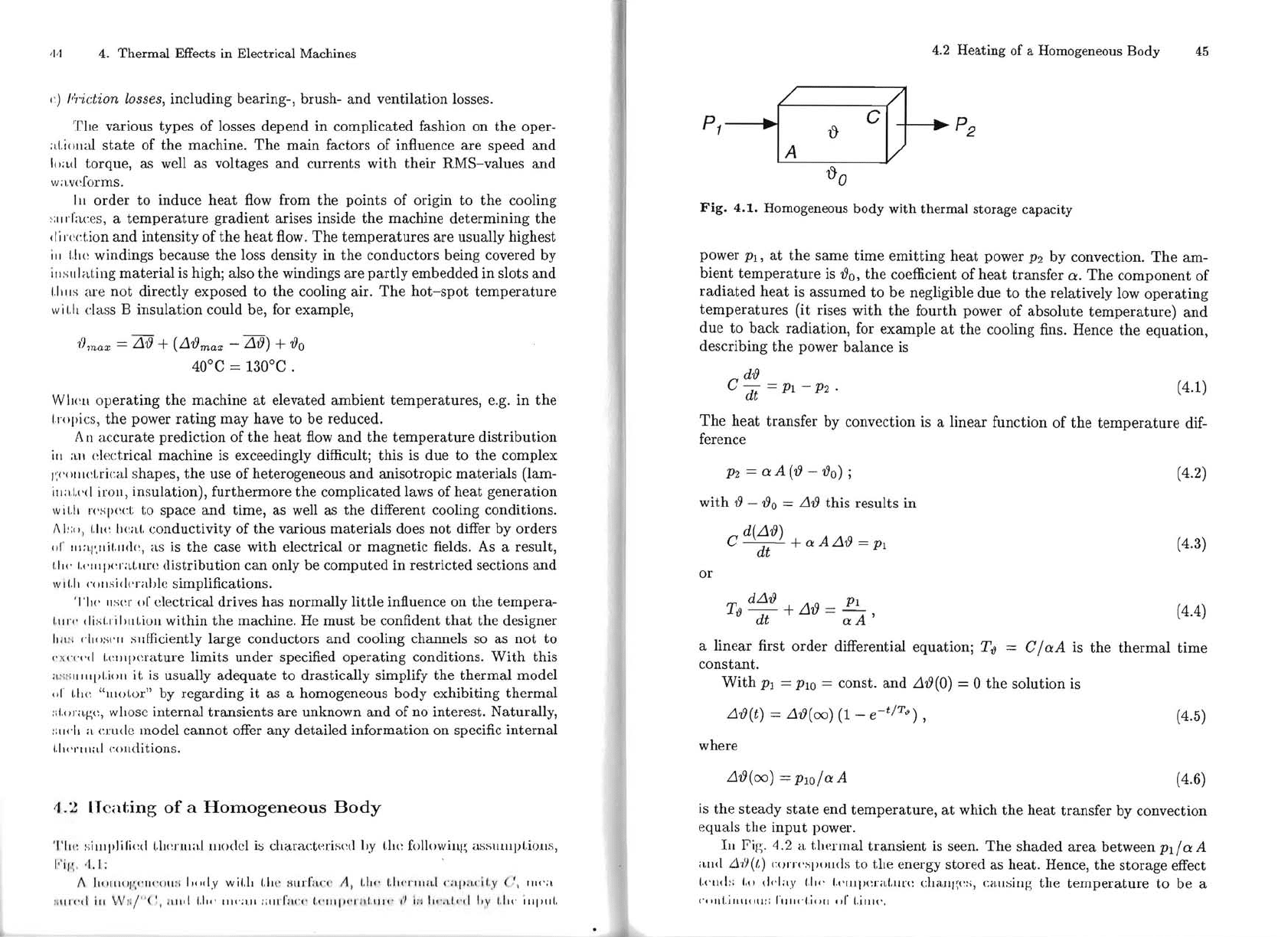
Fir;. 4.2 a

tlwrrnal

transient

is seen.

The

shaded

area

between

pI/a

A

aud

Lh'l(t,)

c()ITI',~p()llds

to

the

energy

stored

as

heat.

Hence,

the

storage

effect

1.1'

11(1:

:

1.11

dc'I:I,)'

1.

11f'

1

.

l'llll)(~l'at.lIn!

chaJlg(!:;, ea.llsiJlp;

the

temperature

to

be

a

(""lIl.illllllll~:

1'11111'1.;1111

III'

1.

;1111',

47

~

ti

4.

Thermal

Effects

in

El

e

ctrical

Machines

P10

L1~

\

I

~

L

W(oo)

=

aA

L1~(O)

Change

of

stored thermal

energy

T

JJ

heating transient

T

JJ

cooling-off transient

Fig.

4.2.

Thermal

transients

The

approximation incurred with this simple model is mainly due to

the

assumption

of

evenly

distributed

heat

sources

in

the

homogeneous

body

and

t\w

Il

eglect

of

an

internal

heat

flow;

hence,

transportation

delays are

not

rOlltained

in

the

simplified model.

A rough

estimate

of a typical

thermallag

may

be

derived from

the

data

sll('d. of

an

enclosed 100

kW

standard

induction

motor

cooled by

an

external

\';\.

1I

(TEFC):

100 k

W,

nominal power

M

~

OO

kg, mass

, I

0.92, nominal efliciency

. I,

,')

('

x

,)

GO

°C

is

the

steady-state

temperature

rise due

to

the

losses

PI

at

)'

/I

11<IIlIill:d

p()w(~r

1'1

1'"

(~-1)

LIli'

C

(l

lI

v(

'

cl.ive

heat conductivity is

PI

Ir

11.

L119(oo)

-:"c

J\

h

S

lllllill~

that

the

motor

consists

of

solid iron having

the

specific

heat

CFe,

I.

!tI

,

hea.L

capacity

is

c =

Cl"e

M.

'I'

hi

s y

idds

the

thermal

time

constant

~

= C/"e M

Ll19(oo)

= 0.48 kWsj kgOC 800 kg 50°C

~

34

mino

"

;'

}

n

11.

.!.::.'L

p . 9 kW

71

11.

'l'y

pi

ra

ll

y,

Lhcl'lllal

Lrll.llsj('lI(.s

ar(:

IIl1l

ch I;!ow(:r I.

hall

d(

,ct. rj(·:t! 01' J11(·('hallica.!

1'1\',

'

1'1.

::

()I'

((1111 ::" , 1.

111'\'"

1

1.1

'

('

(·:

x('(:p\.j(lIl

H :1

111'11

I

II

'

di

/l

l(

1II(1(.tll

·H,

wlll'l'!

' 1.

111'

nr

-

111

:.1.

111"

Wl

ll

d i

JlI'

, Irl

I'

Ji

ui<'d di

,.,·(

·l.Iy

(III

!III

I

lI

li

lllll

,I,I

II

P, dllllt I

UIfI

IJl

IIIIH'IIIII ':I

V('I

'y

4.2

Heating

of

a Homogeneous

Body

little

thermal

storage capacity.

The

following

time

scales are usually valid

with

electrical machines:

electromagnetic mechanical

thermal

transients

0.1 - 100 ms

10

ms -

10

s 10 - 60 min

Travelling wave

phenomena

in

windings are

not

considered; they are faster

yet by several orders of magnitude.

The

large difference

of

more

than

a factor

of 100 between

the

time

scales of mechanical

and

thermal

transients usually

permits

a

separate

treatment

which results

in

considerable simplification.

The

heat

transfer by convection from a ventilated surface depends strongly

on

the

velocity of

the

cooling air;

the

usual range

of

the

transfer coefficient is

a=

50t0500WtCm

2

at

Ll79

=

50

°C this results in a power

flow

by convection

of

P2c

j 2

A = 2.5 to

25

kW

m ;

the

dependence of

the

heat

transfer on

the

velo city of

the

cooling air

has

the

consequence

that

self-cooled motors exhibit

at

standstill a cooling

time

constant

that

is

much longer

than

the

thermal

time

constant

of

the

motor

when running. Larger

motors

operating

at

variable speed

and

load are usually

provided

with

separate

forced cooling, causing

the

motor

speed

to

have

little

effect

on

the

cooling conditions.

To show

that

the

heat

transfer by

radiation

can normally be neglected, a

rough

estimate

of

the

power

flow

by radiation is given for comparison.

A "black

body"

emits

to

the

environment power by

radiation

according

to

Boltzmanns

law,

PR

=

uT

4

,

A

where

2

u =

5.710-

8

W

jK

4

m

is

the

coefficient

ofradiation

and

T

the

absolute

temperature.

With

19

= 70°C,

i.e. T

=

343

K,

the

power

flow

due

to

radiation

is

2

PR

=0.

77kWjm

.

A

This

relatively small

amount

is

further

reduced by inverse radiation. AIso,

the

ra

cli

ation coefficieIlt of a

motor

surface

is

much lower

than

that

of

a "black

hod

y" .

Werner Leonhard Control of Electrical Drives

Подождите немного. Документ загружается.