Alfred DeMaris - Regression with Social Data, Modeling Continuous and Limited Response Variables

Подождите немного. Документ загружается.

• b

 2.2299.

• b

 .0085.

• σ

 .0059.

(a) What percent of variation in the cost-of-living index is accounted for by

the growth rate?

(b) Give the sample estimate of the error (disturbance) variance.

tion slope is zero, and show that they are all the same value, within round-

ing error. What is the conclusion for this test?

(d) Interpret the values of b

and b

(e) Give the value of r

adj

2.11 For the cities dataset, let Y  homicide rate and X  reading quotient. Then

for 54 cities we have:

• x  384.7.

• y  409.3.

• x

 3069.29.

• y

 4564.81.

• xy 2663.45.

• (y  yˆ)

 1268.58 for the regression of Y on X.

(a) Find the OLS prediction equation for the linear regression of Y on X.

(b) Find the correlation between Y and X.

and b

in terms of the variables involved.

(d) Test whether or not there is a signiﬁcant linear relationship between Y and X.

(e) What proportion of the variation in the homicide rate of a city is explained

by its reading quotient here?

(f) What is the estimated average homicide rate for all cities in the popula-

tion having a reading quotient of 7.1241?

2.12 Prove that for any given sample of X and Y values, the OLS estimates b

and

produce the largest r

among all possible estimates for the linear regression

of Y on X.

2.13 Using the computer, regress COLGPA on STUDYHRS in the students dataset

and save the residuals. Then use software (e.g., SAS, SPSS) to test whether

the errors are normally distributed in the population. Missing imputation:

Follow the instructions for Exercise 2.1.

2.14 For the cities dataset, a regression of the homicide rate on the 1980 popula-

tion size for 60 cities produces the following statistics:

• Mean (homicide rate)  7.471.

• Mean (1980 population size)  759.618.

EXERCISES 75

c02.qxd 8/27/2004 2:47 PM Page 75

• Std Dev (homicide rate)  5.151.

• Std Dev (1980 population size)  1473.737.

• r

adj

 .2190.

•SSE 1202.000.

(a) Give the OLS estimates of b

and b

for this regression. (Hint: Derive r

from r

adj

by noting that r

adj

 1  [(n  1)/(n  2)](SSE/TSS). Then use r

to compute b

(b) Give the F statistic for testing whether H

: β

 0. Is it signiﬁcant?

2.15 Regard the following data:

Estimate the simple linear regression of Y on X. In particular:

(a) Give the sample regression equation.

(b) Estimate the variance of the disturbances.

(d) Evaluate the empirical consistency of the model by performing the lack-

of-ﬁt test.

(e)Give r

adj

2.16 For the 416 couples in the couples dataset, the regression of coital frequency

in the past month on the male partner’s age produces the following statistic:

RSS  1996.46395. Given that the sample variance of coital frequency is

37.1435 and the sample variance of male age is 215.50965, do the following:

(a) Find the absolute value of the correlation between coital frequency and

male age.

(b) Find the absolute value of the slope of the regression of coital frequency

on male age.

(d) Perform a test of H

: β

 0 against H

: β

 0 using the t test for the slope.

2.17 Let Z

 ( y  y



)/s

and Z

 (x  x



)/s

. Prove that an OLS regression of Z

results in an intercept estimate of zero and a slope estimate that is the cor-

relation between X and Y.

2.18 Using the computer, verify that the regression of Z

on Z

gives b

 0 and

 r, using the example of the regression of COITFREQ on FEMAGE in

the couples dataset.

Obs. XY Obs. XY

112 663

214 766

3 3 1.5 8 10 2

4 3 2 9 10 4

5 3 5 10 10 6.25

76 SIMPLE LINEAR REGRESSION

c02.qxd 8/27/2004 2:47 PM Page 76

2.19 Prove that for n  3, r

adj

is always smaller than r

. (Hint: Write out the formula

for r

adj

from Exercise 2.14. Then subtract and add SSE/TSS from this formula

and factor appropriately.)

2.20 Regard the following (x,y) values for 10 observations:

Do the following:

(a) Estimate the simple linear regression of Y on X.

(b) Show that high discriminatory power can coexist with empirical incon-

sistency by comparing the r

for this regression with the results of the

lack-of-ﬁt test.

2.21 Changing metrics: If b

and b

are the intercept and slope, respectively, for the

regression of Y on X, prove that the regression of c

Y on c

X, where c

and c

are any two arbitrary constants, results in a sample intercept, b

, equal to c

and a sample slope, b

, equal to (c

2.22 Using the computer, change the metrics of COLGPA and STUDYHRS in

the students dataset as follows. Let MCOLGPA  100(COLGPA) and

MSTUDHRS  STUDYHRS/24. Then verify the principles of Exercise 2.21

by regressing MCOLGPA on MSTUDHRS and comparing the coeﬃcients to

those from the regression of COLGPA on STUDYHRS. Missing imputation:

Follow the instructions for Exercise 2.1.

2.23 Using the computer, regress EXAM1 on STATMOOD in the students dataset

and save the residuals. Then correlate the residuals with STATMOOD, EXAM1,

COLGPA, and SCORE. Also, correlate yˆ with STATMOOD, the residuals, and

EXAM1. Explain the value of each of these correlations. Missing imputation:

Substitute 3.0827835 for missing values on COLGPA and 40.9358974 for miss-

ing values on SCORE.

2.24 Rescaling: If b

and b

are the intercept and slope, respectively, for the regres-

sion of Y on X, prove that the regression of Y  c

on X  c

results in a sam-

ple intercept, b

, equal to b

 c

b

, and a sample slope, b

, equal to b

Then let c

y



and c

x



, and show that this principle subsumes Exercise

2.6(d) as a special case.

2.25 Recall the decomposition of the population variance of Y, assuming that

Y  β

β

X  ε:V(Y)  V(β

 β

X  ε)  V(β

 β

X)  V(ε).

XY XY XY

1 1.5 5 7.5 9 8

1 1.75 5 7.75 9 8.25

3 4.5 7 8

3 4.75 7 8.25

EXERCISES 77

c02.qxd 8/27/2004 2:47 PM Page 77

Note that this equals β

V(X)  V(ε). Show an analogous decomposition for

the sample variance of Y based on the fact that Y  b

 b

X  e.

2.26 Dichotomous independent variables can be used in regression if they are

dummy-coded. This involves assigning a 1 to everyone in the category of

interest (the interest category) and a 0 to everyone who is in the other cate-

gory on X (the contrast category, or omitted group, or reference group). Show

that in the population, the regression of a continuous variable Y on a dummy

variable X results in β

being the conditional mean of Y for those in the group

coded 0 on X, and β

 β

being the conditional mean of Y for those in the

group coded 1 on X (i.e., the interest category).

2.27 Prove that the sample regression of a continuous Y on a dummy variable, X, has

equal to the mean of Y for the contrast category, and b

equal to the mean of

Y for the interest category minus the mean of Y for the contrast category.

(Hint: Let:

• y



 mean of Y for those in the contrast category

• y



 mean of Y for those in the interest category

• π

 proportion of the sample in the interest category

• n

 number of sample cases in the interest category

• n

 number of sample cases in the contrast category

and note that:

• π

x/n

• x  nπ

 n

• y



 (π



 (1  π



• xy (y x  1), that is, the sum of Y for those in the interest category)

2.28 Using the computer, verify the properties associated with the dummy coding

of X. That is, show that b

 ( y



x  0) and b

 ( y



x  1)  ( y



x  0). As the

example, use the regression of CONFLICT on PRESCHDN in the couples

dataset.

78 SIMPLE LINEAR REGRESSION

c02.qxd 8/27/2004 2:47 PM Page 78

CHAPTER 3

Introduction to Multiple Regression

CHAPTER OVERVIEW

In this chapter I introduce the multiple linear regression (MULR) model, building on

the theoretical foundations established in Chapter 2. I begin with an artiﬁcial exam-

ple that illustrates the primary advantages of multiple regression over simple linear

regression (SLR). A fundamental concept, statistical control for another regressor, is

then explicated in some detail. I then formally develop the model and its assumptions,

and discuss estimation via ordinary least squares as well as inferential tests in MULR.

I then explain the problem of omitted-variable bias and deﬁne the three major types

of bias that can occur when key regressors are omitted from the model: confounding,

suppression, and reversal. I also consider the phenomenon of mediation by omitted

variables, which, although not a form of bias, is central to causal modeling. Next I

discuss statistical interaction and the related issue of comparing models across dis-

crete groups of cases. Finally, I return to the issue of assessing empirical consistency

and evaluate a MULR model for scores on the ﬁrst exam for 214 students in intro-

ductory statistics.

EMPLOYING MULTIPLE PREDICTORS

Advantages and Rationale for MULR

Suppose that we have several potential predictors, X

, X

,..., X

, for a given

response variable, Y. Certainly, we could assess the impact of each X

on Y via a series

of SLRs. In fact, if the X’s are all orthogonal—that is, mutually uncorrelated—the

impact, b

, of a given X

will be no diﬀerent in an SLR of Y on X

than in a MULR

of Y on X

and all other K ⫺ 1 predictors. Moreover, R

from the multiple regression

Regression with Social Data: Modeling Continuous and Limited Response Variables,

By Alfred DeMaris

c03.qxd 8/27/2004 2:48 PM Page 79

would simply be the sum of all the individual r

’s from the K diﬀerent SLRs of Y on

each X

. However, unless the data were gathered under controlled conditions (e.g., via

an experiment), the regressors in social data analysis will rarely be orthogonal. Most

of the time they are correlated—sometimes highly so.

With this in mind, there are four primary advantages of MULR over SLR. First, by

including several regressors in the same model, we can counteract omitted-variable

bias in the coeﬃcient for any given X

. Such bias would be present were we to omit

a regressor that is correlated with both X

and a determinant of Y. Second, we can

examine the discriminatory power achieved when employing the collection of regres-

sors simultaneously to model Y. When the X’s are correlated, R

is no longer the sim-

ple sum of r

’s from the SLRs of Y on each X

. R

can be either smaller or larger than

that sum. The ﬁrst two advantages are germane only when regressors are correlated.

However, the next two advantages apply even if the regressors are all mutually

orthogonal. The third advantage of MULR is its ability to model relationships

between Y and X

that are nonlinear, or to model statistical interaction among two or

more regressors. Although interaction is discussed below, a consideration of nonlin-

ear relationships between the X’s and Y is postponed until Chapter 5. The ﬁnal advan-

tage is that in employing MULR, we are able to obtain a much more precise estimate

of the disturbance variance than is the case with SLR. By “precise” I mean an esti-

mate that is as free as possible from systematic inﬂuences and that comes as close as

possible to representing purely random error. The importance of this, as we shall see,

is that it makes tests of individual slope coeﬃcients much more sensitive to real

regressor eﬀects than would otherwise be the case.

Example

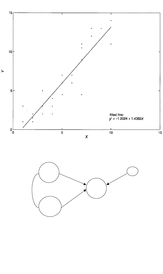
Figure 3.1 presents a scatterplot of Y against X for 26 cases, along with the OLS ﬁtted

line for the linear regression of Y on X. It appears that there is a strong linear impact

of X on Y, with a slope of 1.438 that is highly signiﬁcant ( p ⬍ .0001). For this regres-

sion, the r

is .835, and the estimate of the error variance is 3.003. However, the plot

is somewhat deceptive in suggesting that X has such a strong impact on Y. In truth,

this relationship is driven largely by a third, omitted variable, Z. Z is strongly related

to both Y (r

⫽ .943) and X (r

⫽ .891). If Z is a cause of both Y and X, or even if Z

is a cause of Y but only a correlate of X, the SLR of Y on X leads us to overestimate

the true impact of X on Y, perhaps by a considerable amount. What is needed here is

to control for Z and then reassess the impact of X on Y.

Controlling for a Third Variable

What is meant in this instance by controlling for Z or holding Z constant? I begin

with a mechanical analogy. Figure 3.2 illustrates a three-variable system involving

X, Y, and Z. Actually, there are four variables—counting ε, the disturbance—but only

three that are observed. Suppose that this system is the true model for Y. Further,

imagine that the circles enveloping X, Y, Z, and ε are gears, and the arrows and

80 INTRODUCTION TO MULTIPLE REGRESSION

c03.qxd 8/27/2004 2:48 PM Page 80

curved lines connecting these variables are drive shafts. Running the SLR of Y on X

alone is tantamount to hiding the shaft, γ, that runs from Z to Y. When you turn the

X gear, the Y gear also turns—maybe quite a bit—because X is also connected to Z,

and Z also turns Y. However, since the shaft from Z to Y is hidden, we are misled into

thinking that X’s power to move Y is all realized through the shaft β. What we really

want to know, of course, is how much X turns Y, if at all, just on its own. In such

EMPLOYING MULTIPLE PREDICTORS 81

Figure 3.1 Scatterplot of (x,y) values, along with OLS regression line, depicting the linear relationship

between Y and X for 26 cases.

Figure 3.2 Regression model for Y showing confounding of X–Y relationship due to a third variable, Z.

c03.qxd 8/27/2004 2:48 PM Page 81

a system, one simple solution, of course, is simply to disconnect γ. Then when we

turn X, if Y also turns, we know that this is strictly due to β, not to the other con-

nection through Z. What this solution accomplishes is to stop Z from turning along

with X, so that if turning X turns Y, this can only be due to β. The analogy to vari-

ables and their relationships is made by equating “turning” with variation. We want

to know whether varying X also induces Y to vary, and we don’t want X’s eﬀect to

be confounded with Z’s eﬀect on Y. Hence, we must stop Z from varying along with

X in order to isolate X’s eﬀect on Y.

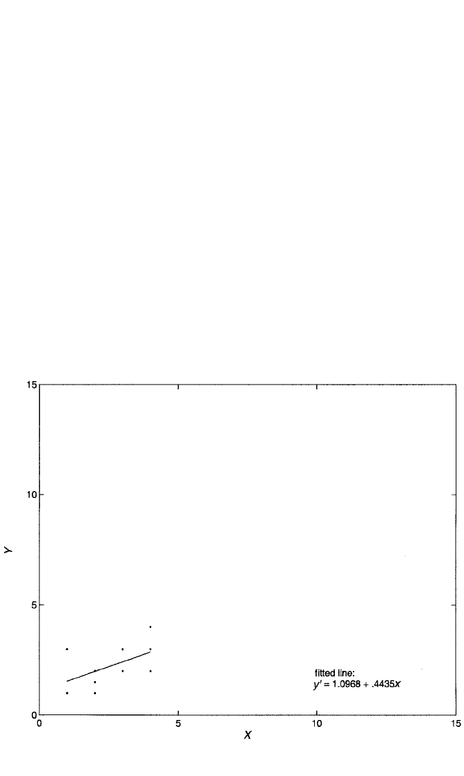
The principle of holding Z constant and observing how much Y varies with X

alone is illustrated, in the current example, in Figures 3.3 to 3.5. The variable Z,

measured for all 26 cases, takes on three values: 1, 2, and 3. Figure 3.3 shows a plot

of Y against X for all cases whose Z-value is 1. Notice that we are literally holding

Z constant in this plot, since all cases have the same value of Z (i.e., Z is no longer

varying here). Also notice that the slope of the regression of Y on X for just these

cases is now much shallower than before, with a value of only .444, about a third of

its previous value achieved when Z was ignored. Figure 3.4 similarly shows a plot of

Y against X for cases whose Z-value is 2. The slope of the regression here is .595.

Finally, Figure 3.5 shows Y plotted against X for those with Z-values of 3. The slope

of the regression in this case is .544.

82 INTRODUCTION TO MULTIPLE REGRESSION

Figure 3.3 Scatterplot of (x,y) values, along with OLS regression line, depicting the linear relationship

between Y and X for the 10 cases with Z-values equal to 1.

c03.qxd 8/27/2004 2:48 PM Page 82

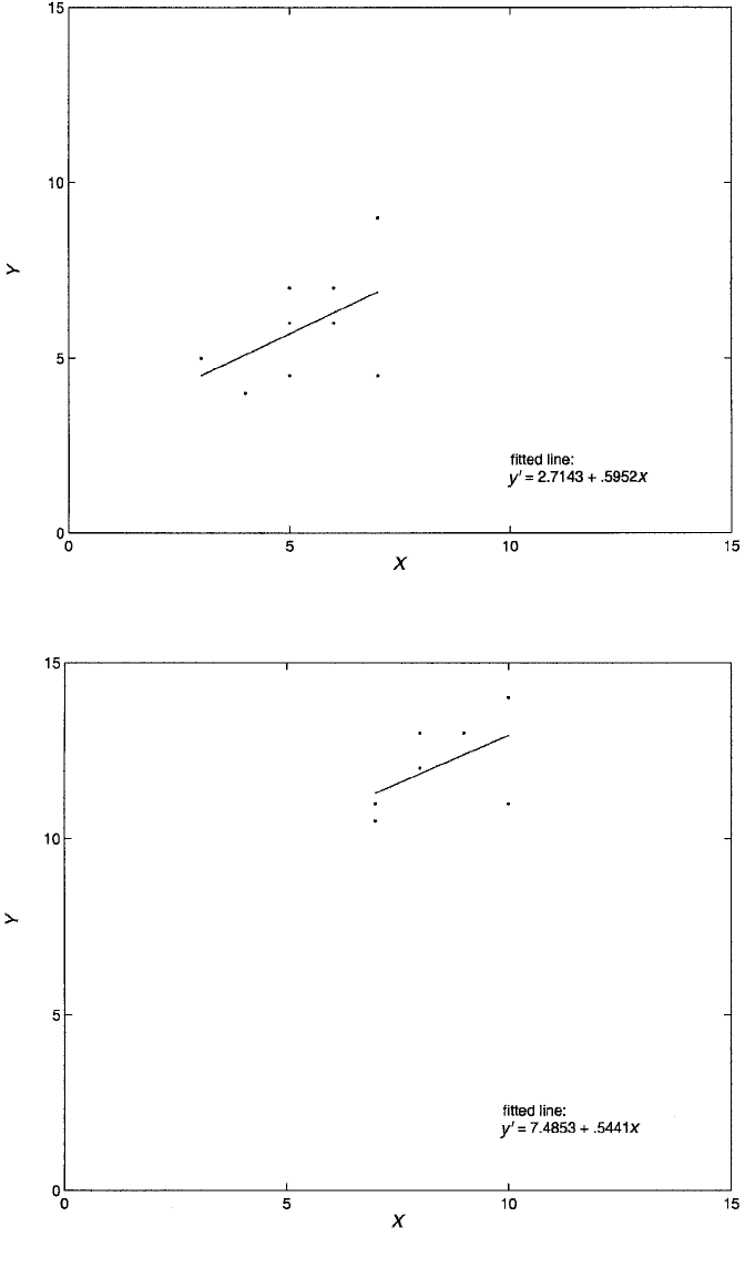
Figure 3.4 Scatterplot of (x,y) values, along with OLS regression line, depicting the linear relationship

between Y and X for the nine cases with Z-values equal to 2.

Figure 3.5 Scatterplot of (x,y) values, along with OLS regression line, depicting the linear relationship

between Y and X for the seven cases with Z-values equal to 3.

c03.qxd 8/27/2004 2:48 PM Page 83

A simple summary of X’s impact on Y when controlling for Z might be obtained

by averaging the three individual X–Y slopes from each level of Z, since their values

are quite similar. This is not exactly the formula used to calculate the eﬀect of X in

the multiple regression of Y on X and Z (see Exercise 3.17 for the correct formula),

but it is a good heuristic approximation. The average of the three slopes is .528.

Hence, we could say that holding Z constant, each unit increase in X is expected to

increase Y by about .528 unit, on average. This is substantially smaller than the slope

of X’s eﬀect on Y when Z is not controlled, which was 1.438. Clearly, failing to con-

trol for Z results in an overestimate of the impact of X. Statistically, controlling for

Z is accomplished by including it, along with X, in the equation for Y and estimat-

ing the MULR model. In the MULR, the slope for X is actually .564 instead of .528;

nonetheless, the reduction in value compared to 1.438 is clear. Additionally, the esti-

mate of the disturbance variance in the MULR is 1.614, or about half that in the

SLR. The error variance in the SLR was obviously inﬂated by not removing the sys-

tematic variance accounted for in Y by Z. Finally, R

in the MULR is .915, compared

to .835 in the SLR. In that X and Z are highly correlated, the R

in the MULR is much

less than the sum of the individual r

’s explained by X and Z in isolation (.835 and

.889, respectively).

A ﬁnal and more formal way of understanding the meaning of statistical control

is as follows. Suppose that we regress X on Z and arrive at the estimated equation:

X ⫽ c ⫹ dZ⫹ u. Now, notice that u ⫽ X ⫺ (c ⫹ dZ). That is, u is the part of X that is

not a linear function of Z. Recall from Chapter 2 that u is also uncorrelated with Z.

Then suppose that we perform the SLR of Y on u and get Y ⫽ a ⫹ bu⫹ e. Then b

from this SLR is exactly the same as the slope of X in the MULR of Y on X and Z.

Here we see that control, once again, is achieved by preventing Z from varying

along with X. In this case, it is evident that such control is achieved by using a form

of X from which the linear association with Z has been removed. Since that form of

X is now orthogonal to Z, b represents the impact of X on Y while preventing Z from

varying along with X, or holding Z constant. (Exercise 3.8 asks you to verify this

principle using the computer to analyze a four-variable model from the students

dataset.)

MULR Model

Now that we understand the need and rationale for MULR, it is time to present the

model and assumptions for estimation via OLS. The MULR model for the ith

response, Y

,is

⫽ β

⫹ β

⫹

...

⫹ β

⫹ ε

. (3.1)

Or, the model for the conditional mean of Y, given the X’s, is

E(Y

冟X

, X

,...,X

) ⫽ β

⫹ β

⫹

...

⫹ β

84 INTRODUCTION TO MULTIPLE REGRESSION

c03.qxd 8/27/2004 2:48 PM Page 84