Alfred DeMaris - Regression with Social Data, Modeling Continuous and Limited Response Variables

Подождите немного. Документ загружается.

Also, the covariance of the residuals with X is

cov(x

)













 0.

The orthogonality condition must be taken on faith. However, the best assurance of

its veracity is to include in one’s model any other determinants of Y that are also cor-

related with X. How to model Y as a function of multiple regressors is taken up in

Chapter 3.

Nonlinearities. Plots of residuals against X are also useful for revealing potential

nonlinearities in the relationship between Y and X. This would be suggested by



i  1

 yˆ

)  x





i  1

 yˆ

)



n  1



i1

x





i1

n1



i1

x



n1



i1

x



)(e

e



)

n1

ASSESSING EMPIRICAL CONSISTENCY OF THE MODEL 65

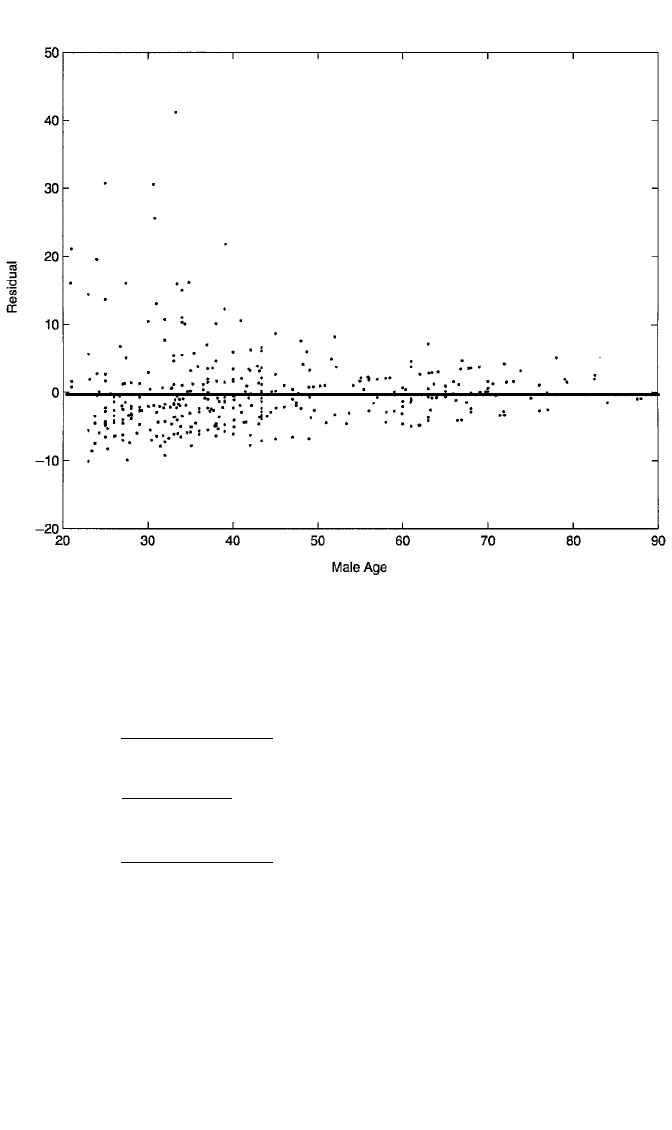
Figure 2.7 Plot of residuals against male partner’s age from OLS regression of couple’s coital frequency

in past month on male partner’s age for 416 couples from the NSFH.

c02.qxd 8/27/2004 2:47 PM Page 65

a point scatter with a nonlinear shape around the line e  0. No such pattern is evi-

dent in the point scatter in Figure 2.6.

Outliers. The diagnosis of unusual observations is taken up in detail in Chapter 6,

but I also consider it brieﬂy here. Although not oﬃcially an assumption of regres-

sion, it is ideal if the data are also free of outliers. These are observations that are

noticeably “out of step” with the trend shown by the majority of the points. An out-

lier typically shows up as an unusually large (in absolute value) residual. Outliers are

essentially observations that are not ﬁt well by the model. At the least, we would like

to identify them. They may show up in an ordinary residual plot, but a better strat-

egy is to plot the standardized residuals against X.

Standardized Residuals. A residual is standardized by subtracting its mean and

dividing by its standard deviation. For this purpose we recall that the mean of the

residuals is zero and that the estimated standard deviation of the equation errors is σ

The standardized residual is therefore z

 (e  0)/σ

 e/σ

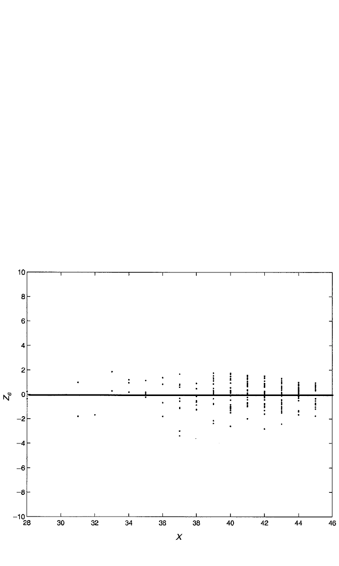
. Figure 2.8 presents a plot

of the standardized residuals against X for the regression of exam 1 performance on

math diagnostic scores. If the equation errors were normally distributed, we might

66 SIMPLE LINEAR REGRESSION

Figure 2.8 Plot of z

(standardized residuals) against X (math diagnostic score) from OLS regression of

score on exam 1 on math diagnostic score for 213 students in introductory statistics.

c02.qxd 8/27/2004 2:47 PM Page 66

want to consider as outliers residuals that are 2 standard deviations or more on

either side of the zero line. However, given that the errors may not be normally dis-

tributed, we should be more cautious. Neter et al. (1985) suggest four or more stan-

dard deviations as the benchmark for extreme residuals. Regarding Figure 2.8, it does

not appear that any particular observations meet this criterion. Most of the z

are well

within this limit, with only two observations approaching it. Above all, however, none

of the points appears dramatically out of step with the rest of the point scatter. (On the

other hand, the observation with the largest magnitude z

, in the lower middle of

the plot, is somewhat of an outlier, as will be pointed out in Chapter 6.)

Formal Test of Empirical Consistency

A lack-of-ﬁt test proposed by Neter et al. (1985) can be employed to formally test

the empirical consistency of the model. In this section I discuss the test and then

employ it to test the empirical consistency of the simple linear regression for exam

scores in Table 2.2. This test assumes normality of the equation errors, in addition to

zero mean and constant variance. The test, according to the authors, is for “ascer-

taining whether or not a linear regression function is a good ﬁt for the data” (Neter

et al., 1985, p. 123). The test generally requires repeated observations at each value

of X, which is not a problem in the current example.

The test is based on a decomposition of SSE into pure error and lack-of-ﬁt com-

ponents. The ﬁrst component, the pure error sum of squares, or SSPE, is the total

variability of the Y-scores around their respective group means at each x. That is,

suppose that there are c diﬀerent X-values. In the regression of exam scores, for

example, there are c  16 diﬀerent math diagnostic scores, ranging from 28 to 45.

Let x

denote the jth X-value and n

denote the number of observations with X  x

Also, let y

denote the ith observation whose X-value is x

, and let y



stand for the

mean of all of the y

whose X-value is x

. Then the sum of squares of Y-values about

their mean at a particular x

is 

i  1





)

. Note that if there is only one observa-

tion at a particular x

, then y

 y



, implying that y

 y



 0. Thus, observations with

unique values of X do not contribute any information to SSPE.

The total such variability across all of the X-values is

SSPE 



j1



i1

 y



)

(2.9)

The pure error mean square (MSPE) is SSPE divided by its degrees of freedom,

which is n  c. Hence,

MSPE 







It turns out that MSPE is an unbiased estimator of the error variance, σ

, regardless

of the nature of the function relating X to Y. For this reason, it is dubbed an estimate

of “pure error.”

ASSESSING EMPIRICAL CONSISTENCY OF THE MODEL 67

c02.qxd 8/27/2004 2:47 PM Page 67

The second component of SSE is the lack-of-ﬁt sum of squares (SSLF). Further

denoting, by yˆ

, the sample-regression ﬁtted value at X  x

, SSLF is

SSLF 



j1



 yˆ

)

This is essentially a weighted (by the n

) sum of squared deviations of the y



from the

regression line. The greater the deviation of the y



from the regression line, the more

evidence that a linear regression does not characterize the conditional mean of Y,

given X (Neter et al., 1985). Conveniently, SSLF can also be calculated as SSE –

SSPE. The degrees of freedom associated with SSLF is c  2. Hence, the lack-of-ﬁt

mean square (MSLF), is

MSLF 







The test statistic for testing for a lack of ﬁt is

F 



Under the null hypothesis that a linear regression model ﬁts the data, or that the data

are empirically consistent with a linear regression, F has the F distribution with c  2

and n  c degrees of freedom.

Implementing the Test. The lack-of-ﬁt test is not currently implemented for the lin-

ear regression model in mainstream software—say in SPSS or SAS. However, it can

be obtained in SAS, since this software implements the test for a response surface

model via the program PROC RSREG. For a regression with one predictor, X,the

response surface model is simply a model that adds X

as another regressor. At any

rate, RSREG calculates and prints SSPE for this quadratic model. Nevertheless, SSPE

is the same as in equation (2.9), since SSPE is always just the deviation of the Y

around

their group means at each x. For the regression of exam performance on math diag-

nostic scores, we have the following: SSE is 45102.50265 and SSPE is 2044.573675.

Therefore, SSLF  SSE  SSPE  45102.50265  2044.573675  43057.928975.

As noted previously, n  213 and c  16. MSPE is thus 2044.573675/197  10.3785,

and MSLF  43057.928975/14  3075.5664. The lack-of-ﬁt test is therefore F 

3075.5664/10.3785  296.34. With 14 and 197 degrees of freedom, the result is highly

signiﬁcant ( p  .00001). I should therefore reject the hypothesis that the data are

empirically consistent with the model.

How troublesome is this ﬁnding? It should be noted, ﬁrst, that in the quadratic

model, it is only the linear eﬀect that is signiﬁcant. That is, the X

term is very

nonsigniﬁcant, suggesting that there is no simple departure from linearity evident in

the regression. Moreover, the scatterplot in Figure 2.1 and the residual plots in

Figures 2.6 and 2.8 all seem to suggest that a linear regression adequately describes

the relationship between exam performance and math diagnostic score. It is possible,

68 SIMPLE LINEAR REGRESSION

c02.qxd 8/27/2004 2:47 PM Page 68

particularly with larger sample sizes, that haphazard departures from linearity may

result in the rejection of empirical consistency. Yet without a clear nonlinear trend

that could be modeled, preserving the linear regression approach may be the best

strategy, from the standpoint of parsimony. In sum, I accept the linear regression

model as appropriate for the data in this example, despite having to reject the hypoth-

esis of empirical consistency via a formal test.

Discriminatory Power vs. Empirical Consistency. As another illustration of the dis-

tinction between discriminatory power and empirical consistency, I conducted a

regression simulation. First, I drew a sample of 200 observations from a true linear

regression model in which Y was generated by the linear equation 3.2  1X  ε, where

ε was normally distributed with mean zero and variance equal to 22. Estimation of the

simple linear regression equation with the 200 sample observations produced an r

.21. The F statistic for testing empirical consistency was .2437. With 8 and 190 degrees

of freedom, its p-value was .982. Obviously, the F test for lack of ﬁt here suggests a

good-ﬁtting model. Note, however, that discriminatory power is modest, at best. Next

I drew a sample of 200 observations from a model in which Y was generated as a

nonlinear—in particular, a quadratic—function of X. Speciﬁcally, the equation generat-

ing Y was 1.2  1X  .5X

 ε. Again, ε was a random observation from a normal dis-

tribution with mean zero. This time, however, the variance of ε was only 1.0. I then used

the 200 sample observations to estimate a simple linear regression equation. That is, I

estimated Y  β

 β

X  ε, a clearly misspeciﬁed model. The test for lack of ﬁt in this

case resulted in an F value of 339.389, a highly signiﬁcant result (at p  .00001).

Clearly, by a formal test, the linear model is rejected as empirically inconsistent. The

for the linear regression, however, was a whopping .96! The point of this exercise is

that contrary to popular conception, r

is not a measure of “ﬁt” of the model to the data.

It is a measure of discriminatory power. It’s possible, as shown in these examples, for

good-ﬁtting models to have only modest r

values and for bad-ﬁtting models to have

very high discriminatory power. [See also Korn and Simon (1991) for another illustra-

tion of the distinction between these two components of model evaluation.]

Authenticity. The authenticity of a model is much more diﬃcult to assess than is

either discriminatory power or empirical consistency. Here we ask: Does the model

truly reﬂect the real-world process that generated the data? This question usually does

not have a statistical answer. We must rely on theoretical reasoning and/or evidence

from experimental studies to buttress the veracity of our proposed causal link between

X and Y. On the other hand, we can evaluate whether additional variables are respon-

sible for the observed X–Y association, rendering the original causal model inauthen-

tic. For example, I have attempted above to argue, theoretically, for the reasonableness

of math diagnostic score as a cause of exam performance, for years of schooling as a

cause of couple modernism, and for frequenting bars as a cause of sexual frequency.

Objections to the authenticity of all of these models can be tendered. With respect to

exam performance, it is certainly possible that academic ability per se is the driving

force that aﬀects performance on both the math diagnostic and the exam. In this case,

the relationship between diagnostic score and exam performance, being due to a third,

ASSESSING EMPIRICAL CONSISTENCY OF THE MODEL 69

c02.qxd 8/27/2004 2:47 PM Page 69

causally antecedent variable, would be spurious. Couple modernism may be deter-

mined strictly by the female’s years of schooling. Its association with male’s years of

schooling, rather than reﬂecting a causal link, may simply be an artifact of the sub-

stantial correlation between each spouse’s educational level. Finally, sexual activity

and going to bars may be associated purely by virtue of the fact that younger people

engage in both activities with greater frequency, rendering the correlation between sex

and bar going, once again, spurious. Fortunately, each of these alternative explanations

for the observed linear associations can be examined given that measures of the addi-

tional variables are available in the data sets. In Chapter 3 I introduce multiple linear

regression, which allows us to examine the relationship between X and Y while con-

trolling for additional factors. I can then assess each of these alternative hypotheses.

For now, I leave these alternative models for the three outcomes as potential competi-

tors for the models underlying the data.

STOCHASTIC REGRESSORS

The assumption of nonstochastic regressors, that is, regressor values that are ﬁxed over

repeated sampling, is quite restrictive. Generally, only in experiments does the

researcher have the power to ﬁx the diﬀerent levels of X at particular values. With non-

experimental data, such as are gathered via surveys of, say, the general population,

what are actually sampled are random observations of (x,y) pairs. In this case, both Y

and X are random, or stochastic, variables. In this situation, it is unreasonable to expect

the X-values to remain constant over repeated sampling. The reason for this is that each

sample may contain a somewhat diﬀerent random sampling of X-values. Nevertheless,

according to Neter et al. (1985), all results articulated earlier, pertaining to estimation,

testing, and prediction, employing the model with ﬁxed X, also apply under random X

if the following two conditions hold: (1) “The conditional distributions of the Y

,given

, are normal and independent, with conditional means β

 β

and conditional vari-

ance σ

”; and (2) “The X

are independent random variables, whose probability distri-

bution g(X

) does not involve the parameters β

, β

, σ

” (Neter et al., 1985, p. 84).

Regardless of whether these conditions hold, the ﬁxed-X assumption is unnecessary

if we are willing to make our results conditional on the sample values observed for

the independent variable. This means that they are valid only for the particular set of

X-values that we have observed in our sample. According to Wooldridge (2000), con-

ditioning on the sample values of the independent variable is equivalent to treating the

as ﬁxed over repeated sampling. Such conditioning then implies automatically that

the disturbances are independent of X, which is the primary requirement for the valid-

ity of our model-based inferences.

ESTIMATION OF

ββ

AND

ββ

VIA MAXIMUM LIKELIHOOD

In this ﬁnal section of the chapter, I show how to arrive at estimates of β

and β

using maximum likelihood rather than OLS estimation. I do this to provide some

consistency in coverage of model estimation, since all models in this book other than

70 SIMPLE LINEAR REGRESSION

c02.qxd 8/27/2004 2:47 PM Page 70

the linear regression model typically rely on maximum likelihood as the estimation

method.

In the appendix to Chapter 1, I discussed maximum likelihood estimation and

provided a relatively simple illustration of the technique. Recall that the key mathe-

matical expression is the log of the likelihood function for the parameters, given the

data. To arrive at this, maximum likelihood estimation begins with an assumption

about the density function of the observed response variable. In this case, we assume

that the equation disturbances have a normal distribution with mean zero and vari-

ance σ

at each x

. Given that the X’s are ﬁxed and that the conditional mean of y

 β

, this means that the y

are normal with mean equal to β

 β

and condi-

tional variance equal to σ

. Hence, the density function for each y

f(y

x

,β

) 



2





exp









 (β

 β

)





which means that the joint density function for the vector y of sample responses,

given the vector x of regressor values, is

f(y x, 

,

) 

i



2





exp









 β





Given the data observed, this becomes a function only of the parameters; hence we

change its symbol to L(β

,β

y,x), indicating that it is the likelihood function for the

parameters, given the data, equal to

L(β

,β

y,x)  (2πσ

)

 n/2

exp











i1

 β

)



Denoting the log of this function by ᐉ(β

, β

y,x), we have

艎(β

,β

y,x) 



ln 2πσ





2σ





i1

 β

)

. (2.10)

Recall from the earlier discussion of least squares estimation that ﬁnding the values

of variables that minimize or maximize a function involves setting the ﬁrst deriva-

tives of the function, with respect to each of the variables, to zero and then solving

the resulting simultaneous equations. In this case, with the variables b

and b

sub-

stituted for the parameters, we have



∂



[艎(β

,β

y,x)] 





i1

 b

)

and



∂



[艎(β

,β

y,x)] 





i1

 b

ESTIMATION OF β

AND β

VIA MAXIMUM LIKELIHOOD 71

c02.qxd 8/27/2004 2:47 PM Page 71

Now, these expressions are zero whenever



i1

 b

)  0 and



i1

 b

)  0.

Notice that these are just the normal equations that were solved to ﬁnd the least

squares estimates. This shows that the OLS estimates, b

and b

, are also the maxi-

mum likelihood estimates if the Y

are normally distributed. Moreover, it is easy to

convince ourselves that this solution, in fact, maximizes the log likelihood. Recall the

argument supporting b

and b

as minimizing SSE. Now notice that ᐉ(β

, β

y,x) is

generally a negative value, so to maximize it we have to ﬁnd the values that make it

least negative. Obviously, this occurs whenever SSE is minimized. In this case, the

second negative expression on the right-hand side of equation (2.10), which is a

function of SSE, reaches its least negative value, and therefore ᐉ(β

, β

y,x) attains

its maximum.

EXERCISES

2.1 Using the computer, regress EXAM1 on COLGPA in the students dataset.

Missing imputation: substitute the value 3.0827835 for missing data on COL-

GPA. Then:

(a) Interpret the values of b

and b

(b) Give the values of σ

and σ

(d) Give the values of r

and r

adj

(e) Give the estimate of σ

(f) Give the predicted population mean of Y for those with a college GPA of

3.0.

(g) Give a 95% conﬁdence interval for β

2.2 Using the computer, regress STATMOOD on SCORE in the students dataset.

Missing imputation: Substitute the value 40.9358974 for missing data on

SCORE. Then:

(a) Interpret the values of b

and b

(b) Give the values of σ

and σ

(d) Give the values of r

and r

adj

(e) Give the estimate of σ

(f) Give the predicted population mean of Y for those with a math diagnostic

score of 43.

(g) Give a 95% conﬁdence interval for β

2.3 Consider the regression of coital frequency on male age for our 416 couples.

How reasonable is the orthogonality assumption? That is, are there any

72 SIMPLE LINEAR REGRESSION

c02.qxd 8/27/2004 2:47 PM Page 72

compelling theoretical reasons why you would expect the disturbances to be

correlated with male age in the population?

2.4 Regard the following (x,y) values for 19 observations:

(a) Construct a scatterplot of Y against X.

(b) Estimate the regression of Y on X and draw the regression line on the plot.

sion on just the ﬁrst 18 observations.

(d) How does the regression change, and what seems to account for the change?

2.5 Prove, for simple linear regression, that the point x



, y



is on the regression line.

2.6 A centered variable, X

, is deﬁned as X

 X  X



. Do the following:

(a) Prove that centering X leaves the slope unchanged in SLR.

(b) Prove that centering X makes the intercept equal to y



in SLR.

advantage to centering X in simple linear regression?

(d) Suppose that we center both X and Y; that is, let Y

 Y  Y



and X

 X  X



Now, for the regression of Y

on X

, show that the slope is again unchanged

but that the intercept is now zero.

2.7 Using the computer, verify the properties associated with centering both Y and

X, using the regression of COITFREQ on FEMAGE in the couples dataset.

2.8 A random sample of six students was drawn from a large university to deter-

mine if depression is related to GPA. Depression was measured with the

Center for Epidemiologic Studies Depression Scale (CESD). This particular

short version of the scale ranges from 0 to 84, with higher scores indicating

more depressive symptomatology. The researchers think that students with

lower GPAs suﬀer more from depression because they are more worried

about their future job or graduate school prospects. Summary statistics are:

• Mean (GPA)  3.

• Mean(CESD)  50.

• Std Dev(GPA)  .894.

• Std Dev(CESD)  28.284.

• cov(GPA,CESD) 20.

XY XY X Y X Y

1 .5 2 1.7 4 1.3 10 1

1 1 3 .4 4 2 10 2.5

1 1.5 3 1.2 5 .6 10 4

2.6 35 52 1018

2 1 4 .7 5 2.2

EXERCISES 73

c02.qxd 8/27/2004 2:47 PM Page 73

(a) Give the regression equation for predicting CESD from GPA.

(b) Give the correlation coeﬃcient for the correlation of CESD with GPA.

dent, based on the sample regression.

2.9 Regard the following data:

Student SAT GPA Student SAT GPA Student SAT GPA

1 4.8 2.4 5 3.8 2.7 9 7.2 3.4

2 6.6 3.5 6 5.2 2.4 10 6.0 3.2

3 5.9 3.0 7 6.6 3.0

4 7.4 3.8 8 5.0 2.8

To determine which incoming students should receive scholarships, a univer-

sity admissions oﬃcer decided to study the relationship between a student’s

score on the SAT verbal test (taken in the ﬁnal year of high school) and the

student’s college GPA at the end of the sophomore year. Ten student records

for juniors at the university were examined. The data are shown above. The

SAT scores have been divided by 100. The oﬃcer reasoned that if SAT scores

are strongly related to GPA, an incoming student’s SAT score gives a good

indication of how well he or she will do in college.

(a) How strong is the relationship between GPA and SAT?

(b) Is this relationship signiﬁcant?

(d) Using this equation, what is the predicted GPA for the ﬁrst student?

(e) What is the residual for the ﬁrst student?

2.10 The cities dataset consists of data compiled by the author on a random sam-

ple of 60 of the largest U.S. cities as of 1980. Several characteristics of these

cities, based on 1980 census data, were measured, including:

• Homicide rate: number of homicide victims per 100,000 population.

• Cost-of-living index: the average market value of houses divided by average

household income.

• City growth rate: percent increase in population from 1970 to 1980.

• Population size: the number of inhabitants of the city, in thousands of persons.

• Reading quotient: the total number of volumes, plus daily volume circula-

tion, across all libraries in the city, divided by population size.

A simple linear regression of the cost-of-living index on the city growth rate

produces the following sample statistics for 60 cities:

• r  .18453.

• SSE  34.8798.

• RSS  1.2296.

74 SIMPLE LINEAR REGRESSION

c02.qxd 8/27/2004 2:47 PM Page 74