Amaro A., Reed D., Soares P. (editors) Modelling Forest Systems

Подождите немного. Документ загружается.

23Amaro Forests - Chap 20 25/7/03 11:08 am Page 226

226 V. Alenius et al.

When modelling and classifying mortality it is necessary to determine to what

extent causality and regularities are taken into account and what phenomena are

regarded as stochastic. Subsequently, mortality can be classiﬁed as regular (non-

catastrophic) or irregular (catastrophic) (Vanclay, 1995). Regular mortality reﬂects

lowering vigour and decreasing growth rate, which may originate from ageing or

lack of resources and increasing competition and, as such, is at least partially pre-

dictable (Murty and McMurtrie, 2000). Irregular mortality is typically caused by

storms, forest ﬁres, epidemics of pathogenes or insect population explosions, where

the survival probability is unpredictable at tree level but not necessarily at land-

scape level. Several logistic mortality models accounting for regular tree-level mor-

tality mainly due to competition have been developed (e.g. Monserud, 1976;

Hamilton, 1986; Avila and Burkhart, 1992; Monserud and Sterba, 1999; Shen et al.,

2000; Eid and Tuhus, 2001; Yao et al., 2001). Such models are mainly applied to con-

trol the predicted stocking level in stand simulators (e.g. Crookston, 1990; Botkin,

1993; Van Dyck, 2001; Hynynen et al., 2002).

It is common for individual tree mortality data to include several stands with

mor

e than one tree in each stand. As a consequence, the observations (trees in the

same stand) are always correlated. This fact has generally not been accounted for in

modelling individual tree mortality, although it calls for different methods of model

construction, and consequently leads to different procedures in parameter estima-

tion. Ignoring data structure in two- or more level mortality data leads to, for exam-

ple, too small standard errors for higher-level ﬁxed effects which are measured at

plot or stand levels, a problem similar to any multivariate normal regression of

multilevel data. Therefore, when logistic regression is applied to multilevel data,

methods of analysis and measures of model ﬁt which are appropriate especially for

these situations should be seriously considered. In this study, we compared logistic

mortality models for peatland Scots pine (Pinus sylvestris L.), which were developed

both with and without random stand effect and by alternative estimation methods

using two-level data. We discussed the methods of parameter estimation and the

use of different goodness-of-ﬁt measures in the case of correlated data.

State of the Art

Traditional logistic regression

In logistic regression (Hosmer and Lemeshow, 2001), the dependent variable may be

binary or expr

essed in proportions. With the logit transformation, the linear model

is as follows

()





1 −

()



αβ

(1)

()

= ln











αβ

where

(x) =

is an intercept and

is a vector of unknown parameters.

1 + e

αβ

The distribution of the errors is supposed to be binomial with zero mean and vari-

ance

(x)[1

(x)]. The error term has two possible values: if E(y) = 1 then

= 1

(x)

with probability

(x), and if E(y) = 0 then

= 

(x) with probability 1

(x). The

conditional distribution of y follows the binomial distribution with probability

given by the conditional mean,

(x).

The maximum likelihood (ML) method is used to estimate the parameters of

the logistic r

egression model, because the unknown parameters are non-linearly

23Amaro Forests - Chap 20 25/7/03 11:08 am Page 227

227 Logistic Regression in Modelling Mortality

related to

(x). The model’s statistical evaluation is done on the basis of several cri-

teria developed to guide in choosing the best model from different candidates.

Assessing the ﬁt is usually done with the Pearson

statistic and the deviance. The

Hosmer–Lemeshow test looks for the correctness of the model in grouping probabil-

ities in risk deciles. The classiﬁcation table describes the model’s goodness of ﬁt

with the correct classiﬁcation rate. The receiver operating characteristic (ROC) curve

(Hosmer and Lemeshow, 2001) is based on sensitivity and speciﬁcity measures. A

high ROC curve describes the good prediction ability of the model. The area under

the curve is interpreted as the model’s R

Multilevel logistic regression with random effect

Multilevel logistic regression models for hierarchically structured data have become

mor

e common in recent studies of social sciences and medicine (e.g. Hox, 1995;

Goldstein and Rasbash, 1996; Carlin et al., 1999; Fielding, 2000). Forestry applica-

tions are few (Jalkanen, 2001), and published tree mortality models, for example,

have been constructed from multilevel data, but in parameter estimation the data

structure has been ignored.

Multilevel binary data can be analysed using a logistic regression model which

is composed of ﬁxed covariates fr

om different hierarchy levels and random effects

(Hosmer and Lemeshow, 2001; McCulloch and Searle, 2001). The random effects not

related to the lowest level of hierarchy are generally assumed to follow normal dis-

tribution with mean zero and constant variance. Here the random stand effect

describes the unmeasured variance between the stands in case of mortality. The

error variance (tree-level variance) is assumed to be:

(2)

φπ

()

(

−

()

)

where

is the dispersion scale (or extra-binomial variance). If

= 1, then the error

variance is purely binomial. If

> 1, the situation is called over-dispersion. Unlike

under-dispersion (

< 1), over-dispersion is fairly common, and may occur when

data are collected from experiments with a hierarchical design (McCullagh and

Nelder, 1989). If the dispersion scale is forced to be equal to 1, the potential over-

dispersed variance is added to the random effect variance.

The ML and restricted maximum likelihood (REML) methods are relevant

when analysing linear multilevel models with normal distribution, but logistic

egression models with random effects need special quasi-likelihood estimation

methods. The key point is to estimate the effect of the covariates on the binary out-

come with awareness of the random effect(s). The idea of quasi-likelihood methods

is that only the model for the mean (response and covariates) and the relationship

between the mean and the variance is necessary for the estimation. Two quasi-likeli-

hood methods have been developed for estimation: the marginal quasi-likelihood

(MQL) and the penalized quasi-likelihood (PQL) methods. Today these methods are

available in most statistical software packages. However, Rodriguez and Goldman

(1995) have pointed out that in certain circumstances the ﬁrst-order MQL estimates

are badly biased, sometimes more biased than those obtained by ML without ran-

dom effects. The PQL method has also been noticed to have a major problem in

practice if the cluster size is small (McCulloch and Searle, 2001). Alternatives to the

ML approach are, for instance, GEE, generalized estimating equations (Zeger et al.,

1988) or Bayesian methods (MCMC, bootstrapping) (e.g. Goldstein, 1995; Browne

and Draper, 2002), which will not be addressed in this chapter.

23Amaro Forests - Chap 20 25/7/03 11:08 am Page 228

228 V. Alenius et al.

There is a basic problem with the goodness-of-ﬁt measures in the case of multi-

level logistic regression; all tests based on likelihood are approximations, because

the likelihood is also an approximation. According to Hosmer and Lemeshow

(2001), many of the goodness-of-ﬁt statistics have not been evaluated for hierarchi-

cal data, but they do recommend some of these tests instead of dismissing any

model checking.

Methodology

Multilevel model

In this study, the response variable is binary, i.e. the observed responses y

of the tree

status may have two values: 0 = live or 1 = dead. With the standard assumptions of

the dependent variable, the distribution for the response is y

∼

Bin(1,

) with bino-

mial variance

(1

), where

is the probability of the jth tree to die in stand i.

A two-level model with a random effect can be written in the general form:

βµ

)

= logit

()

+ X

+ u

i (3)

(

ij 0 ij

where

is as above, term X

is the component of the linear predictor, which has

ﬁxed coefﬁcients (i.e. tree diameter at breast height, basal area of larger trees divided

by stand basal area, stand basal area, proportion of birch of total basal area, qua-

dratic mean diameter), and u

represents random departure from the average proba-

bility for a tree to die in the ith stand at logit scale. As stated earlier, the random

variable u is normally distributed with zero mean and variance σ

. The residual

error variance is a function of

as in Equation 2.

Estimation

The log-likelihood function for the logistic regression with random effect is deﬁned

as follows:

∞



(

+ x

)





exp







−





()

∑

∫



∏

1 + e

+ x





(4)

0 i

i =1

−∞







For multilevel binary models, the quasi-likelihood method is attractive in para-

meter estimation due to its ability to generate highly efﬁcient estimators

(McCulloch and Searle, 2001). The MQL method utilizes the score functions of log-

likelihood as the model for the mean and the model for the relationship between

mean and variance. This is not a very reasonable way to estimate the variance–

covariance matrix, because in the hierarchical collected data there is a correlation

between observations. In MQL this relationship between mean and variance is

based on an assumption of equal variance (simple variance–covariance structure),

which is not always reasonable. Goldstein and Rasbash (1996) showed that

improved estimation is obtained by applying the second-order PQL method, in

which the second-order Taylor expansion for the random part is calculated based

on current residuals u

with variance–covariance matrix D. The corresponding

equations for

are:

∂

MQL =

∑

= 0

∂

(5)

and

23Amaro Forests - Chap 20 25/7/03 11:08 am Page 229

229 Logistic Regression in Modelling Mortality

∂

′

− 1

PQL =

∑

−

u D u = 0 (6)

∂ 2

where Q

is constructed using only information about how the variance changes as

− t

a function of the mean.

∫

τϑ

(

)

, where

is a constant of proportionality

relating var(y

) to the linear predictor variance

(

To demonstrate the differences that result from ignoring the data structure in

the analysis, we ﬁrst estimated the standar

d logistic regression model with maxi-

mum likelihood for 5-year mortality. In the multilevel analysis, ﬁrst-order MQL and

second-order PQL methods (Goldstein and Rasbash, 1996) were used. The tree-level

error variance was also tested for over- and under-dispersion (Goldstein, 1995). All

parameters of the multilevel logistic models were estimated simultaneously. We

used

SAS (SAS Institute, 1994) and MLwiN (Goldstein et al., 1998) software to estimate

the models.

Goodness of ﬁt

In traditional logistic regression, the difference between observed and ﬁtted values

is measur

ed with Pearson residuals:

)

(

y − m

)

(7)

ˆ ˆ

(

l −

)

where y

denotes the number of dead trees among m subjects with x

covariates. The

ﬁtted values yˆ

= m

in logistic regression are calculated for every independent vari-ˆ

able and are called the covariate patterns m

j = 1, 2,…, J. The Pearson

test is based

on adjusted residuals.

∑

r y

)

(8)

(

j = 1

– under the assumption that the ﬁtted model is correct – follows

distribu-

tion with degrees of freedom equal to J(p+1), where p is the number of

parameters. It should be noticed that in

, y

is considered as a relative fre-

quency and m

is assumed to be large. One of the goodness-of-ﬁt measures is

deviance, which is based on so-called adjusted deviance residuals. The differ-

ence between the likelihood of saturated and estimated models, the likelihood

ratio test, is equal to deviance and also follows

distribution. However, it is only

an approximation.

The Hosmer–Lemeshow test groups the estimated probabilities from smallest to

lar

gest into groups (g), which are called the ‘deciles of risk’. The Hosmer–Lemeshow

goodness-of-ﬁt C

is based on the Pearson

test from the g × 2 table of observed and

estimated expected frequencies:

(

− n



)

(9)

k k

C =

∑



(

l −

)

k = 1

where n

is the total number of subjects in the kth group, c

denotes the number of

covariate patterns in the kth group,

o =

∑

is the number of responses among c

j= 1

23Amaro Forests - Chap 20 25/7/03 11:08 am Page 230



230 V. Alenius et al.

covariate patterns, and

∑

is the average estimated probability. C

j=1

approximated by the

distribution with g  2 degrees of freedom. Evans (1998,

cited in Hosmer and Lemeshow, 2001) has shown that with some restrictions the test

can be applied to correlated data.

The classiﬁcation table is an informative way to describe the results. The model

predicts the continuous probabilities; to convert these back to dichotomous results a

cutpoint (c) must be deﬁned. If the estimated probability is less than c, the outcome

value is 0; otherwise it is 1. One way to determine the cutpoint is to choose it in such

a way that the rate of correct classiﬁcation is maximized. The rate of correct classiﬁca-

tion can be determined as the sum of the diagonal elements of the classiﬁcation table

divided by the total number of observations.

Sensitivity and speciﬁcity can be obtained fr

om the classiﬁcation table. These

measures describe how correct the model is in classifying dead and living trees.

Sensitivity is the frequency of observed ‘1’ which the model predicted as ‘1’ divided

by all observed ‘1’. Speciﬁcity is the frequency of observed ‘0’, which the model has

predicted as ‘0’, divided by all observed ‘0’. Evaluating the cutpoint in such a way

that sensitivity and speciﬁcity are as high as possible, the estimated probabilities in

risk deciles frequency should have large frequencies close to 0 and 1. Sensitivity and

speciﬁcity form the basis of describing the model’s ROC curve, which is drawn as

sensitivity against (1speciﬁcity) with all possible cutpoints. The height of the curve

describes the model’s ability to predict the phenomenon. The area under the curve

represents the model’s R

We calculated

, the classiﬁcation table, speciﬁcity, sensitivity, bias, the

Hosmer–Lemeshow test, ROC curves and R

as the basis of evaluation and dis-

cussed their use for this purpose in multilevel data. The bias was calculated in two

ways: (i) tree-level bias as the average difference of tree-level mortality observations

and predictions, and (ii) stand-level bias as an average difference of stand-level

observed and predicted mortalities.

Data

We used the permanent peatland growth plots (SINKA) as the modelling data. The

SINKA stand is composed of a cluster of three circular plots located 40 m apart. In

order to avoid too-laborious measurements in dense sapling stands, the radii of the

circular sample plots were adjusted according to the stand density in such a way

that the whole SINKA cluster contained approximately 100 tally trees. For those, the

minimum diameter at breast height (DBH) was 4.5 cm if the stand was past pole

age, and 2.5 cm otherwise. The ﬁrst re-measurement of the SINKA data was done in

1988–1994 following a period of ﬁve growing seasons on each plot. For a more

detailed description of the data, see, for example, Hökkä et al. (1997). From the struc-

ture of the data, it is clear that trees within stands are correlated.

For the purposes of this study, both pure Scots pine and mixed pine–birch

stands (an admixtur

e of Betula pubescens Ehrh.) were included in the data if at least

one pine was present in the cluster. The data were restricted to stands where no

management operations (thinning, ditching) had been carried out during the last

5-year period preceding the ﬁrst measurement or between the measurement occa-

sions. Altogether, the numbers of stands and trees were 295 and 17,293, respec-

tively. The mortality proportion for pine was 2.73%. The average tree DBH for

23Amaro Forests - Chap 20 25/7/03 11:08 am Page 231

231 Logistic Regression in Modelling Mortality

pine was 9.1 cm (range 2.5–44.5 cm). The proportion of large trees in the data was

low; there were only 27 pines with DBH larger than 30 cm.

Results and Discussion

Model assumptions and estimation methods

In the basic logistic regression approach without random variable (ML), the

assumption of independent r

esiduals was violated. This can be seen in the lower

values of the standard errors of stand-level variables compared with those of the

multilevel models (Table 20.1). The parameter estimates were not far from those of

the multilevel models, the greatest difference being in the coefﬁcients of DBH

1

and

DW (18% and 16% underestimates compared with the MQL estimates, but the dif-

ference was non-signiﬁcant when the standard errors were considered). In the MQL

estimation, the tree-level variable DBH

1

inﬂuenced mortality more when com-

pared with the basic logistic regression, while the opposite was true with the stand-

level variables. The variance component related to the between-stand variation in

mortality was clearly signiﬁcant in all multilevel models. The advantage of the

model with random effect (MQL and PQL) is that the model can be calibrated to a

speciﬁc stand, if mortality from the preceding 5-year period has been observed (see

McCulloch and Searle, 2001). For a more detailed description of the construction

and interpretation of the models, see Jutras et al. (2003).

For the multilevel models, the MQL and PQL estimation methods also showed

somewhat dif

ferent results (Table 20.1). There was no problem of convergence with

PQL, which has been the case in many other studies. In our data, PQL estimates in

the ﬁxed part were always larger than MQL estimates, but the difference was statis-

tically signiﬁcant only for G, stand basal area (m

/ha). The opposite was true for the

random stand effect. This suggested that with MQL, less variation was accounted

for by the ﬁxed part. With MQL, minor overdispersed variation was detected. When

the scale effect was ﬁxed at 1 in MQL, the overdispersed variance was transformed

to the between-stand variance. With PQL, the assumption of binomial variance

appeared to be valid in our data.

Table 20.1. Models for peatland Scots pine mortality estimated by different methods. Standard errors

are given in parentheses.

Models

1st order MQL, 2nd order PQL,

ML, without with extra with extra

Variables

random effect 1st order MQL dispersion 2nd order PQL dispersion

Constant 5.719 (0.307) 5.855 (0.465) 4.515 (0.227) 6.808 (0.515) 6.808 (0.515)

DBH

–1

30.884 (10.553) 37.64 (12.78) 37.155 (13.356) 42.1 (14.731) 42.098 (14.736)

BALRAT 2.091 (0.319) 2.020 (0.355) 2.027 (0.373) 2.137 (0.403) 2.137 (0.403)

G 0.111 (0.010) 0.107 (0.022) 0.108 (0.021) 0.132 (0.023) 0.132 (0.023)

G_B 2.133 (0.231) 2.007 (0.435) 2.011 (0.434) 2.170 (0.474) 2.170 (0.474)

DW 0.128 (0.024) 0.110 (0.043) 0.112 (0.043) 0.125 (0.046) 0.125 (0.046)

 1.985 (0.231) 1.842 (0.197) 1.579 (0.251) 1.579 (0.251)

Dispersion 1.000 (0.000) 1.000 (0.000) 1.112 (0.012) 1.000 (0.000) 1.001 (0.011)

scale

DBH

1

, tree diameter at breast height (mm); BALRAT, basal area of larger trees/stand basal area; G,

stand basal area, (m

/ha); G_B, proportion of birch of total basal area (%); and DW, quadratic mean

diameter (cm).

Browne and Draper (2002) pointed out that in many cases both MQL and PQL

methods produce clearly biased parameter estimates, PQL being generally more rec-

ommendable than MQL. Differences in estimates became evident in situations

where the number of observations within clusters was small (see McCulloch and

Searle, 2001). According to Goldstein and Rasbash (1996), the low number of obser-

vations at the lowest level and especially the ratio of the level-1 units to level-2 units

may be the main source of bias in estimates. It is clear that with few observations the

estimation of covariance parameters is unstable. This is also the case with PQL, as

shown by Browne and Draper (2002). In our data, the ratio (average number of trees

in stand : number of stands) was 59 : 295, and was probably sufﬁcient, since all the

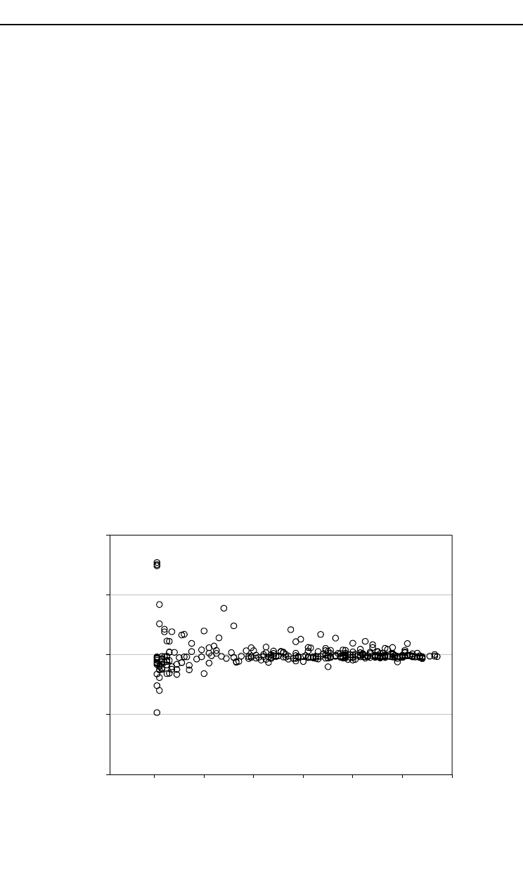
methods appeared to give parameter estimates that were close to each other. Figure

20.1 illustrates the effect of cluster size on estimates with the help of the difference of

stand-wise-calculated average mortality and corresponding predicted probability.

Figure 20.1 shows that when the number of trees per stand is less than 30, there is

large variability in residuals. When there are fewer than 10 trees per cluster, the

residuals may be anything between 0.0 and ±0.8. In a way this is trivial in data

where the average probability is low, because for clusters with a low number of

observations, one tree is representing high relative proportion in such clusters. The

model, however, predicts low probabilities in these stands, too.

Another factor that has been assumed to inﬂuence the ﬁrst-order MQL esti-

mates is the magnitude of the higher-level variance. This was not a problem with

our data either, despite the fact that the two-level variance was relatively high

(1.6–2.0) compared with the value of 0.5 which Rodriguez and Goldman (1995) and

Goldstein and Rasbash (1996) gave as the limit for large variance.

In cases where PQL and MQL appear to give biased results, both Goldstein

(1999) and Browne and Draper (2002) suggest the use of Bayesian methods.

However, these are computationally much more demanding (Browne and Draper,

2002).

232 V. Alenius et al.

Number of trees in stand

0 20406080100120

–1.0

–0.5

0.0

0.5

1.0

Stand-level residual

Fig. 20.1. Stand-level mortality residuals (average observed mortality in the stand – average predicted (MQL

method) probability) as a function of the number of trees in the stand.

23Amaro Forests - Chap 20 25/7/03 11:08 am Page 232

23Amaro Forests - Chap 20 25/7/03 11:08 am Page 233

233 Logistic Regression in Modelling Mortality

Fitting measures

The logistic regression goodness-of-ﬁt measures are generally based on Pearson

esiduals and deviance. They can be used only with the assumption of the indepen-

dence of observations. In hierarchical data, the residuals are correlated in clusters,

i.e. stands, so these ﬁtting measures are biased and may be used only for specula-

tion. T

able 20.2 shows a lot of instability in the Pearson

test among different mod-

els. As discussed by Hosmer and Lemeshow (2001), Evans (1998) has improved the

Pearson

test to make it applicable to correlated data, but we are not able to con-

sider it in more detail here.

The classiﬁcation table can be used as an overall measure of goodness-of-ﬁt also

in cases of corr

elated data, since it is not affected by the data structure. The result of

the ordinary Hosmer–Lemeshow test is not reliable because it is assuming indepen-

dence among the observations. According to the results, these models did not ﬁt

into the data.

Our multilevel mortality models appeared to be more speciﬁc than sensitive.

Sensitivity was highest with ML, followed by MQL, and lowest with the PQL

method. Mortality models need to be sensitive, i.e. mor

e accurate, to ﬁnd dead trees

than living ones. With all models there were always some living trees predicted as

dead. With PQL, the rate of correct classiﬁcation was highest (73%), but it predicted

Table 20.2. Goodness-of-ﬁt measures calculated on the basis of the ﬁxed part of the models.

Models

Measure of ﬁt ML 1st order MQL 2nd order PQL

Pearson X

15149.87 19079.26 17306.53

Hosmer–Lemeshow 44.7 45.1 233.9

P value χ

(<0.0001) (<0.0001) (<0.0001)

Sensitivity (%) 73.7 64.2 60.2

Speciﬁcity (%) 56.2 69.1 73.5

Rate of correct 56.7% 68.5% 73.1%

classiﬁcation

Area under the ROC 0.7434 0.7462 0.7291

curve (R

)

Tree-level bias +0.00031 0.00104 +0.01105

Relative (%) +1.1 -3.8 +40.5

Stand-level bias +0.001572 +0.001392 +0.01901

Relative (%) +3.0 +2.8 +36.5

Tree-level bias :

∑

(

−

)

bias

where y

= tree j status, 0 or 1 in stand i;

= predicted probability that tree j in stand i will die; and N =

total number of tree observations.

Stand-level bias :

−

∑

(

)

bias

where Y

= observed mortality in stand i,

∑

; Y

= predicted mortality in stand i,

∑

; S = total

number of stands in data; and n

= total number of trees in stand.

23Amaro Forests - Chap 20 25/7/03 11:08 am Page 234

234 V. Alenius et al.

living trees more accurately than dead ones, resulting in clearly lower sensitivity

than ML and MQL. With MQL, the rate of correct classiﬁcation was 68%, but it pre-

dicted dead trees more accurately than the PQL method.

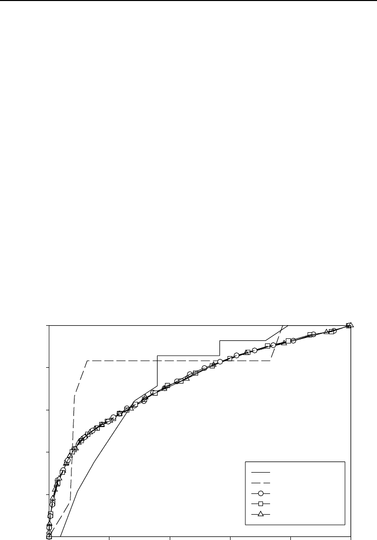
The ROC curve can also be used to select the best model in correlated data,

because it is based on sensitivity and speciﬁcity

. Visually, the curves differed

upwards from the 45° straight line, indicating that the models had rather good abil-

ity to predict tree mortality, but there was virtually no difference among curves (Fig.

20.2). However, the area under the curve (R

) was highest for the MQL method and

lowest for the PQL method (Table 20.2). This suggested that the model obtained by

the MQL method had the highest discrimination ability. Stand-wise-calculated ROC

curves illustrated the model’s (MQL) ability to predict dead trees in speciﬁc stands

in the data (Fig. 20.2).

The logistic model (ML) without random effect gave the lowest tree-level bias,

which is to be expected because it is a population average model and should work

well mar

ginally. The stand-level bias was lowest for the MQL method, which is a

cluster-speciﬁc model accounting for the hierarchical data structure and should

work well at cluster (stand) level.

In general, to be chosen as the best model, all measures need to be good. The

MQL

and ML methods appeared to result in models with good ﬁt measures, accept-

able bias and high R

. Because the MQL method is theoretically correct, the corre-

sponding model should be chosen. The reasons for the poor performance of the PQL

model remain unclear, but the result is not necessarily unusual (see discussion in

McCulloch and Searle, 2001). Here it may be partly due to the strongly skewed data,

with low overall mortality.

Sensitivity

1.0

0.8

0.6

0.4

0.2

0.0

Stand 864 (MQL)

Stand 33 (MQL)

MQL-method

Logistic model

PQL-method

Stand 33

Stand 864

0.0 0.2 0.4 0.6 0.8 1.0

1-Specificity

Fig. 20.2. T

he average ROC curves of different models. Additional curves are drawn for two example

stands, 33 and 864 (on the basis of the MQL method).

23Amaro Forests - Chap 20 25/7/03 11:08 am Page 235

235 Logistic Regression in Modelling Mortality

Conclusions

Our results suggest that with relatively balanced data the marginal quasi-likelihood

(MQL) method produced consistent model estimates for multilevel binary mortality

models. However, the model’s goodness-of-ﬁt is problematic to measure in corre-

lated binary data. The classiﬁcation tables, speciﬁcity, sensitivity, correct classiﬁca-

tion rate, bias and R

may be used to evaluate the model’s performance. Applying

the traditional Hosmer–Lemeshow statistics cannot be recommended. Here the test

suggested rejection of all models, although the models produced by the ML and

MQL methods behaved well in terms of sensitivity, the correct classiﬁcation rate,

and bias. Compared with the other measures, which actually measure the marginal

performance of the models, the ROC curve analyses the predicted probability distri-

bution, and thus is better at describing the variability in the predictions. The graphi-

cal expression did not give additional information to make a selection among the

models, but the R

showed that the models obtained by the ML and MQL methods

were slightly better than that obtained by the PQL method.

When the binary multilevel models are applied, the continuous outcome pre-

dicted by the ﬁxed part is back-transformed into binary values. If the overall cut-

point is applied, the data str

ucture will not be utilized in selecting ‘1’s and ‘0’s.

However, in stand simulators the model can be used in a deterministic way

(Hynynen et al., 2002). The stem frequencies of each DBH class will be decreased by

the amount of the predicted continuous mortality probability, i.e. it is not necessary

to specify a cutpoint and determine which individual will die.

Acknowledgement

We wish to thank Dr Juha Lappi for his valuable comments.

References

Avila, O.B. and Burkhart, H.E. (1992) Modeling survival of loblolly pine trees in thinned and

unthinned plantations. Canadian Journal of Forest Research 22, 1878–1882.

Botkin, D.B. (1993) Forest Dynamics: an Ecological Model. Oxford University Press, Oxford,

309 pp.

Browne, W.J. and Draper, D. (2002) A comparison of Bayesian and likelihood methods for ﬁt-

ting multilevel models. Journal of the Royal Statistical Society, submitted.

Carlin, J.B., Wolfe, R., Coffey, C. and Patton, G.C. (1999) Analysis of binary outcomes in longi-

tudinal studies using weighted estimating equations and discrete time survival methods:

prevalence and incidence of smoking in an adolescent cohort. Statistics in Medicine 18,

2655–2679.

Crookston, N.L. (1990) User’s Guide to the Event Monitor: Part of Prognosis Model Version 6. USDA

Forest Service, Intermountain Research Station, Odgen, Utah, General Technical Report

INT-275, 21 pp.

Dobbertin, M. and Biging, G.S. (1998) Using the non-parametric classiﬁer CART to model for-

est tree mortality. Forest Science 44, 507–516.

Eid, T. and Tuhus, E. (2001) Models for individual tree mortality in Norway. Forest Ecology and

Management 154, 69–84.

Evans, S.R. (1998) Goodness-of-ﬁt in two models for clustered binary data. PhD thesis,

University of Massachusetts at Amherst, Amherst, Massachusetts, 145 pp.

Fielding, A. (ed.) (2000) Generalized Linear Mixed Models in Multilevel and Other Complex Data

Structures in the Social Sciences. Social Science Methodology in the New Millennium.