Anderson D.R., Sweeney D.J., Williams T.A. Essentials of Statistics for Business and Economics
Подождите немного. Документ загружается.

6.1 Uniform Probability Distribution 235
As noted in the introduction, for a continuous random variable, we consider proba-
bility only in terms of the likelihood that a random variable assumes a value within a
specified interval. In the flight-time example, an acceptable probability question is:
What is the probability that the flight time is between 120 and 130 minutes? That is, what
is P(120 x 130)? Because the flight time must be between 120 and 140 minutes
and because the probability is described as being uniform over this interval, we feel
comfortable saying P(120 x 130) .50. In the following subsection we show that
this probability can be computed as the area under the graph of f(x) from 120 to 130
(see Figure 6.2).
Area as a Measure of Probability
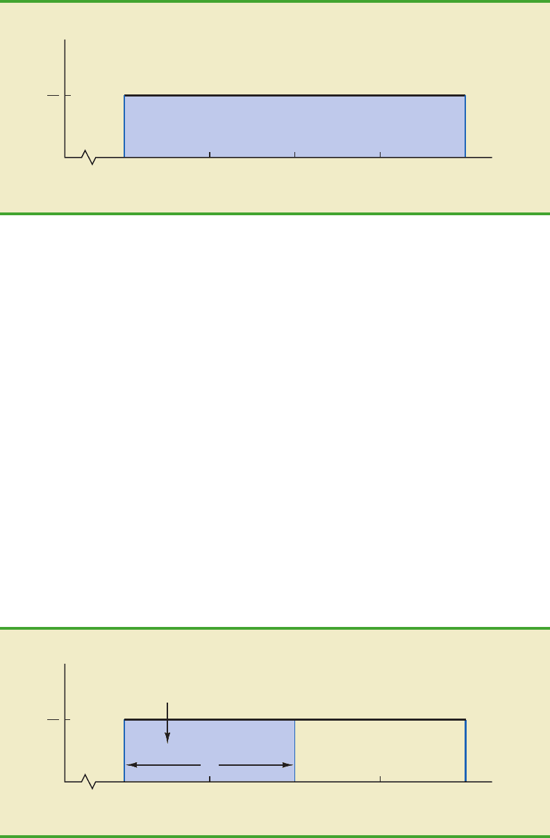
Let us make an observation about the graph in Figure 6.2. Consider the area under the graph
of f(x) in the interval from 120 to 130. The area is rectangular, and the area of a rectangle
is simply the width multiplied by the height. With the width of the interval equal to 130
120 10 and the height equal to the value of the probability density function f(x) 1/20,
we have area width height 10(1/20) 10/20 .50.
Flight Time in Minutes
120 125 130 135 140
x
f (x)
1
20
FIGURE 6.1 UNIFORM PROBABILITY DISTRIBUTION FOR FLIGHT TIME
Flight Time in Minutes
120 125 130 135 140
x
f (x)
1
20
P(120 ≤ x ≤ 130) = Area = 1/20(10) = 10/20 = .50
10
FIGURE 6.2 AREA PROVIDES PROBABILITY OF A FLIGHT TIME BETWEEN 120
AND 130 MINUTES
CH006.qxd 8/16/10 6:34 PM Page 235
Copyright 2010 Cengage Learning. All Rights Reserved. May not be copied, scanned, or duplicated, in whole or in part. Due to electronic rights, some third party content may be suppressed from the eBook and/or eChapter(s).
Editorial review has deemed that any suppressed content does not materially affect the overall learning experience. Cengage Learning reserves the right to remove additional content at any time if subsequent rights restrictions require it.

What observation can you make about the area under the graph of f(x) and probability?
They are identical! Indeed, this observation is valid for all continuous random variables.
Once a probability density function f(x) is identified, the probability that x takes a value be-
tween some lower value x
1
and some higher value x
2
can be found by computing the area
under the graph of f(x) over the interval from x
1
to x
2
.
Given the uniform distribution for flight time and using the interpretation of area as
probability, we can answer any number of probability questions about flight times. For
example, what is the probability of a flight time between 128 and 136 minutes? The width
of the interval is 136 128 8. With the uniform height of f(x) 1/20, we see that
P(128 x 136) 8(1/20) .40.
Note that P(120 x 140) 20(1/20) 1; that is, the total area under the graph of
f(x) is equal to 1. This property holds for all continuous probability distributions and is the
analog of the condition that the sum of the probabilities must equal 1 for a discrete proba-
bility function. For a continuous probability density function, we must also require that
f(x) 0 for all values of x. This requirement is the analog of the requirement that f(x) 0
for discrete probability functions.
Two major differences stand out between the treatment of continuous random variables
and the treatment of their discrete counterparts.
1. We no longer talk about the probability of the random variable assuming a particu-
lar value. Instead, we talk about the probability of the random variable assuming a
value within some given interval.
2. The probability of a continuous random variable assuming a value within some
given interval from x
1
to x
2
is defined to be the area under the graph of the proba-
bility density function between x
1
and x
2
. Because a single point is an interval of
zero width, this implies that the probability of a continuous random variable as-
suming any particular value exactly is zero. It also means that the probability of a
continuous random variable assuming a value in any interval is the same whether or
not the endpoints are included.
The calculation of the expected value and variance for a continuous random variable is anal-
ogous to that for a discrete random variable. However, because the computational proce-
dure involves integral calculus, we leave the derivation of the appropriate formulas to more
advanced texts.
For the uniform continuous probability distribution introduced in this section, the for-
mulas for the expected value and variance are
In these formulas, a is the smallest value and b is the largest value that the random variable
may assume.
Applying these formulas to the uniform distribution for flight times from Chicago to
New York, we obtain
The standard deviation of flight times can be found by taking the square root of the vari-
ance. Thus, σ 5.77 minutes.
Var(x)
(140 120)
2
12
33.33
E(x)
(120 140)
2
130
Var(x)
(b a)
2
12
E(x)
a b
2
236 Chapter 6 Continuous Probability Distributions
To see that the probability
of any single point is 0,
refer to Figure 6.2 and
compute the probability
of a single point, say,
x 125. P(x 125)
P(125 x 125)
0(1/20) 0.
CH006.qxd 8/16/10 6:34 PM Page 236
Copyright 2010 Cengage Learning. All Rights Reserved. May not be copied, scanned, or duplicated, in whole or in part. Due to electronic rights, some third party content may be suppressed from the eBook and/or eChapter(s).
Editorial review has deemed that any suppressed content does not materially affect the overall learning experience. Cengage Learning reserves the right to remove additional content at any time if subsequent rights restrictions require it.

6.1 Uniform Probability Distribution 237
NOTES AND COMMENTS
To see more clearly why the height of a probability
density function is not a probability, think about a
random variable with the following uniform proba-
bility distribution.
f
(x)
再
2
0
for 0 x .5
elsewhere
The height of the probability density function, f(x),
is 2 for values of x between 0 and .5. However, we
know probabilities can never be greater than 1.
Thus, we see that f(x) cannot be interpreted as the
probability of x.
Exercises
Methods
1. The random variable x is known to be uniformly distributed between 1.0 and 1.5.
a. Show the graph of the probability density function.
b. Compute P(x 1.25).
c. Compute P(1.0 x 1.25).
d. Compute P(1.20 x 1.5).
2. The random variable x is known to be uniformly distributed between 10 and 20.
a. Show the graph of the probability density function.
b. Compute P(x 15).
c. Compute P(12 x 18).
d. Compute E(x).
e. Compute Var(x).
Applications
3. Delta Air Lines quotes a flight time of 2 hours, 5 minutes for its flights from Cincinnati to
Tampa. Suppose we believe that actual flight times are uniformly distributed between
2 hours and 2 hours, 20 minutes.
a. Show the graph of the probability density function for flight time.
b. What is the probability that the flight will be no more than 5 minutes late?
c. What is the probability that the flight will be more than 10 minutes late?
d. What is the expected flight time?
4. Most computer languages include a function that can be used to generate random numbers.
In Excel, the
RAND function can be used to generate random numbers between 0 and 1. If
we let x denote a random number generated using
RAND, then x is a continuous random
variable with the following probability density function.
a. Graph the probability density function.
b. What is the probability of generating a random number between .25 and .75?
c. What is the probability of generating a random number with a value less than or
equal to .30?
d. What is the probability of generating a random number with a value greater than .60?
e. Generate 50 random numbers by entering RAND() into 50 cells of an Excel
worksheet.
f. Compute the mean and standard deviation for the random numbers in part (e).
f(x)
再
1
0
for 0 x 1
elsewhere
test
SELF
test
SELF
CH006.qxd 8/16/10 6:34 PM Page 237
Copyright 2010 Cengage Learning. All Rights Reserved. May not be copied, scanned, or duplicated, in whole or in part. Due to electronic rights, some third party content may be suppressed from the eBook and/or eChapter(s).
Editorial review has deemed that any suppressed content does not materially affect the overall learning experience. Cengage Learning reserves the right to remove additional content at any time if subsequent rights restrictions require it.

238 Chapter 6 Continuous Probability Distributions
5. The driving distance for the top 100 golfers on the PGA tour is between 284.7 and 310.6
yards (Golfweek, March 29, 2003). Assume that the driving distance for these golfers is
uniformly distributed over this interval.
a. Giveamathematicalexpressionfortheprobabilitydensityfunctionofdrivingdistance.
b. What is the probability that the driving distance for one of these golfers is less than
290 yards?
c. What is the probability that the driving distance for one of these golfers is at least
300 yards?
d. What is the probability that the driving distance for one of these golfers is between
290 and 305 yards?
e. How many of these golfers drive the ball at least 290 yards?
6. On average, 30-minute television sitcoms have 22 minutes of programming (CNBC,
February 23, 2006). Assume that the probability distribution for minutes of programming
can be approximated by a uniform distribution from 18 minutes to 26 minutes.
a. What is the probability that a sitcom will have 25 or more minutes of programming?
b. What is the probability that a sitcom will have between 21 and 25 minutes of
programming?
c. What is the probability that a sitcom will have more than 10 minutes of commercials
or other nonprogramming interruptions?
7. Suppose we are interested in bidding on a piece of land and we know one other bidder is
interested.
1
The seller announced that the highest bid in excess of $10,000 will be accepted.
Assume that the competitor’s bid x is a random variable that is uniformly distributed
between $10,000 and $15,000.
a. Suppose you bid $12,000. What is the probability that your bid will be accepted?
b. Suppose you bid $14,000. What is the probability that your bid will be accepted?
c. What amount should you bid to maximize the probability that you get the
property?
d. Suppose you know someone who is willing to pay you $16,000 for the property. Would
you consider bidding less than the amount in part (c)? Why or why not?
6.2 Normal Probability Distribution
The most important probability distribution for describing a continuous random variable is
the normal probability distribution. The normal distribution has been used in a wide va-
riety of practical applications in which the random variables are heights and weights of
people, test scores, scientific measurements, amounts of rainfall, and other similar values.
It is also widely used in statistical inference, which is the major topic of the remainder of
this book. In such applications, the normal distribution provides a description of the likely
results obtained through sampling.
Normal Curve
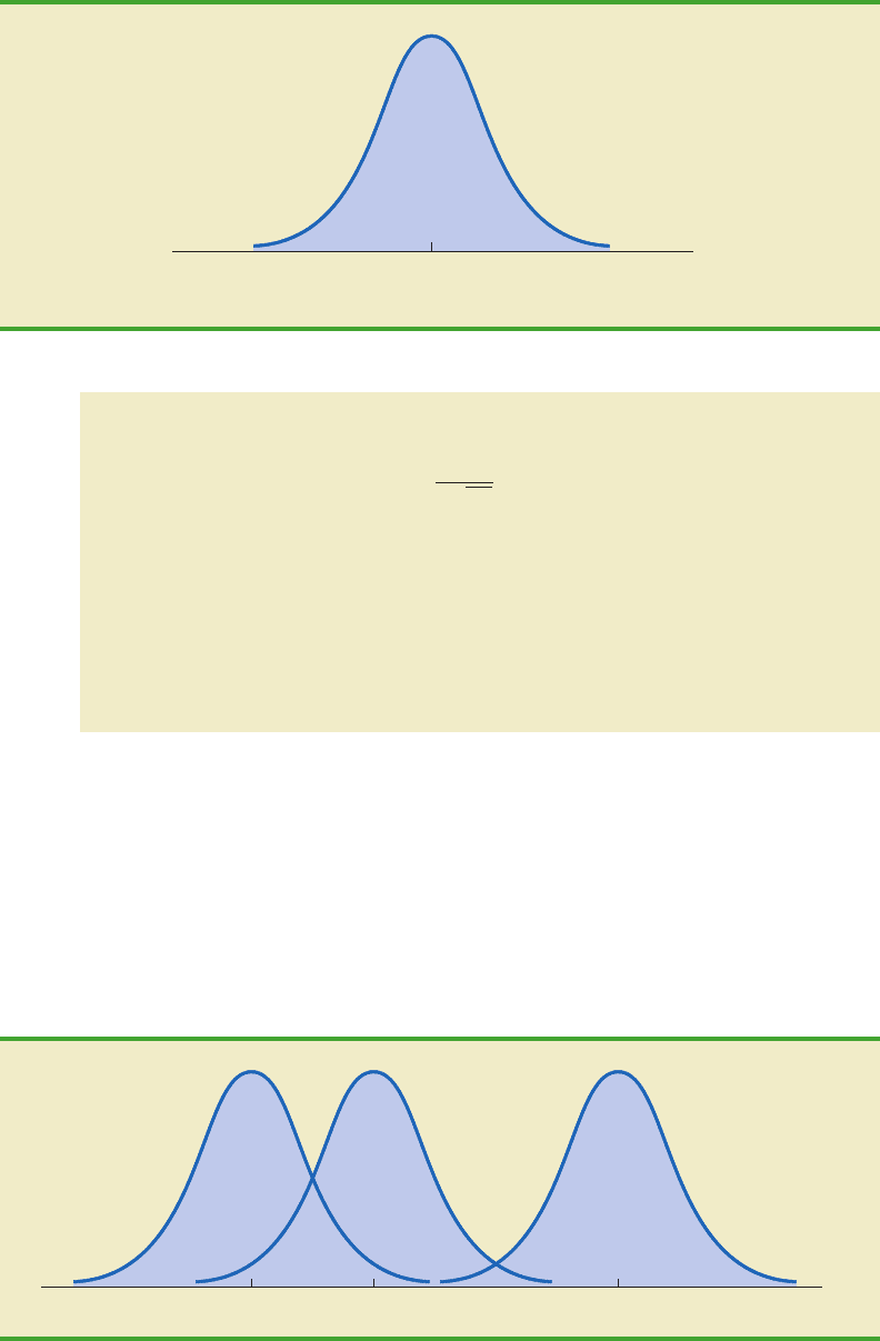
The form, or shape, of the normal distribution is illustrated by the bell-shaped normal curve
in Figure 6.3. The probability density function that defines the bell-shaped curve of the nor-
mal distribution follows.
Abraham de Moivre, a
French mathematician,
published The Doctrine of
Chances in 1733. He
derived the normal
distribution.
1
This exercise is based on a problem suggested to us by Professor Roger Myerson of Northwestern University.
CH006.qxd 8/16/10 6:34 PM Page 238
Copyright 2010 Cengage Learning. All Rights Reserved. May not be copied, scanned, or duplicated, in whole or in part. Due to electronic rights, some third party content may be suppressed from the eBook and/or eChapter(s).
Editorial review has deemed that any suppressed content does not materially affect the overall learning experience. Cengage Learning reserves the right to remove additional content at any time if subsequent rights restrictions require it.
6.2 Normal Probability Distribution 239
NORMAL PROBABILITY DENSITY FUNCTION
(6.2)
where
μ
σ
π
e
mean
standard deviation
3.14159
2.71828
f(x)
1
σ
兹
2
π
e
(xμ)
2
兾2σ
2
We make several observations about the characteristics of the normal distribution.
1. The entire family of normal distributions is differentiated by two parameters: the
mean μ and the standard deviation σ.
2. The highest point on the normal curve is at the mean, which is also the median and
mode of the distribution.
3. The mean of the distribution can be any numerical value: negative, zero, or positive.
Three normal distributions with the same standard deviation but three different
means (10, 0, and 20) are shown here.
The normal curve has two
parameters, μ and σ. They
determine the location and
shape of the normal
distribution.
Mean
x
μ
Standard Deviation s
FIGURE 6.3 BELL-SHAPED CURVE FOR THE NORMAL DISTRIBUTION
–10 0 20
x
CH006.qxd 8/16/10 6:34 PM Page 239
Copyright 2010 Cengage Learning. All Rights Reserved. May not be copied, scanned, or duplicated, in whole or in part. Due to electronic rights, some third party content may be suppressed from the eBook and/or eChapter(s).
Editorial review has deemed that any suppressed content does not materially affect the overall learning experience. Cengage Learning reserves the right to remove additional content at any time if subsequent rights restrictions require it.
240 Chapter 6 Continuous Probability Distributions
4. The normal distribution is symmetric, with the shape of the normal curve to the left
of the mean a mirror image of the shape of the normal curve to the right of the mean.
The tails of the normal curve extend to infinity in both directions and theoretically
never touch the horizontal axis. Because it is symmetric, the normal distribution is
not skewed; its skewness measure is zero.
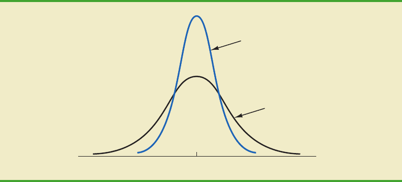
5. The standard deviation determines how flat and wide the normal curve is. Larger
values of the standard deviation result in wider, flatter curves, showing more vari-
ability in the data. Two normal distributions with the same mean but with different
standard deviations are shown here.
6. Probabilities for the normal random variable are given by areas under the normal
curve. The total area under the curve for the normal distribution is 1. Because the
distribution is symmetric, the area under the curve to the left of the mean is .50 and
the area under the curve to the right of the mean is .50.
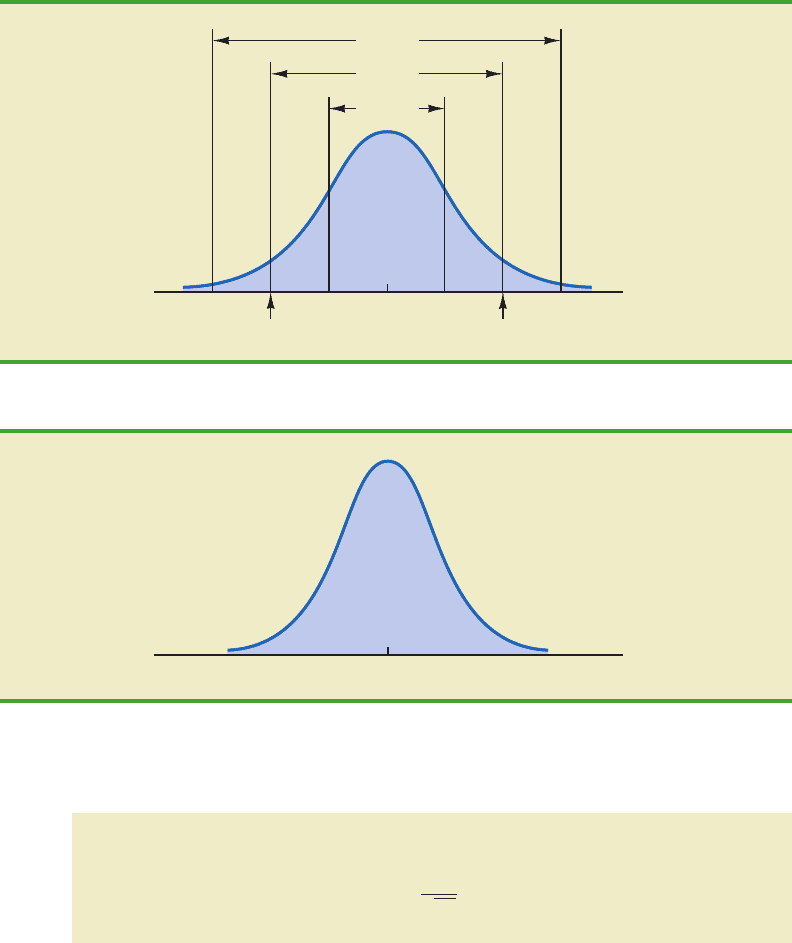
7. The percentage of values in some commonly used intervals are
a. 68.3% of the values of a normal random variable are within plus or minus one
standard deviation of its mean.
b. 95.4% of the values of a normal random variable are within plus or minus two
standard deviations of its mean.
c. 99.7% of the values of a normal random variable are within plus or minus three
standard deviations of its mean.
Figure 6.4 shows properties (a), (b), and (c) graphically.
Standard Normal Probability Distribution
A random variable that has a normal distribution with a mean of zero and a standard devi-
ation of one is said to have a standard normal probability distribution. The letter z is
commonly used to designate this particular normal random variable. Figure 6.5 is the graph
of the standard normal distribution. It has the same general appearance as other normal dis-
tributions, but with the special properties of μ 0 and σ 1.
These percentages are the
basis for the empirical rule
introduced in Section 3.3.
x
μ
σ
= 5
σ
= 10
CH006.qxd 8/16/10 6:34 PM Page 240
Copyright 2010 Cengage Learning. All Rights Reserved. May not be copied, scanned, or duplicated, in whole or in part. Due to electronic rights, some third party content may be suppressed from the eBook and/or eChapter(s).
Editorial review has deemed that any suppressed content does not materially affect the overall learning experience. Cengage Learning reserves the right to remove additional content at any time if subsequent rights restrictions require it.
6.2 Normal Probability Distribution 241
As with other continuous random variables, probability calculations with any normal
distribution are made by computing areas under the graph of the probability density func-
tion. Thus, to find the probability that a normal random variable is within any specific
interval, we must compute the area under the normal curve over that interval.
For the standard normal distribution, areas under the normal curve have been computed
and are available in tables that can be used to compute probabilities. Such a table appears on
the two pages inside the front cover of the text. The table on the left-hand page contains areas,
or cumulative probabilities, for z values less than or equal to the mean of zero. The table on
the right-hand page contains areas, or cumulative probabilities, for z values greater than or
equal to the mean of zero.
Because μ 0 and σ 1, the formula for the standard normal probability density func-
tion is a simpler version of equation (6.2).
STANDARD NORMAL DENSITY FUNCTION
f(z)
1
兹
2π
e
z
2
/2
For the normal probability
density function, the height
of the normal curve varies
and more advanced
mathematics is required to
compute the areas that
represent probability.
x
μ
μ
+ 3 s
68.3%
95.4%
99.7%
μ
+ 2 s
μ
+ 1 s
μ
– 1 s
μ
– 2 s
μ
– 3 s
FIGURE 6.4 AREAS UNDER THE CURVE FOR ANY NORMAL DISTRIBUTION
0
z
= 1
σ
FIGURE 6.5 THE STANDARD NORMAL DISTRIBUTION
CH006.qxd 8/16/10 6:34 PM Page 241
Copyright 2010 Cengage Learning. All Rights Reserved. May not be copied, scanned, or duplicated, in whole or in part. Due to electronic rights, some third party content may be suppressed from the eBook and/or eChapter(s).
Editorial review has deemed that any suppressed content does not materially affect the overall learning experience. Cengage Learning reserves the right to remove additional content at any time if subsequent rights restrictions require it.
242 Chapter 6 Continuous Probability Distributions
The three types of probabilities we need to compute include (1) the probability that the
standard normal random variable z will be less than or equal to a given value; (2) the proba-
bility that z will be between two given values; and (3) the probability that z will be greater
than or equal to a given value. To see how the cumulative probability table for the standard
normal distribution can be used to compute these three types of probabilities, let us consider
some examples.
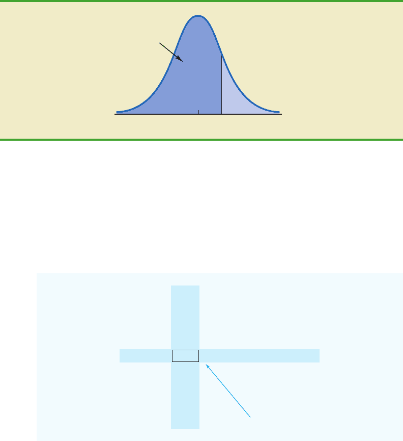
We start by showing how to compute the probability that z is less than or equal to 1.00;
that is, P(z 1.00). This cumulative probability is the area under the normal curve to the left
of z 1.00 in the following graph.
Because the standard
normal random variable is
continuous, P(z 1.00)
P(z 1.00).
Refer to the right-hand page of the standard normal probability table inside the front
cover of the text. The cumulative probability corresponding to z 1.00 is the table value
located at the intersection of the row labeled 1.0 and the column labeled .00. First we find
1.0 in the left column of the table and then find .00 in the top row of the table. By look-
ing in the body of the table, we find that the 1.0 row and the .00 column intersect at the
value of .8413; thus, P(z 1.00) .8413. The following excerpt from the probability table
shows these steps.
z .00 .01 .02
.
.
.
.9 .8159 .8186 .8212
1.0 .8438 .8461
1.1 .8643 .8665 .8686
1.2 .8849 .8869 .8888
.
.
.
P(z 1.00)
.8413
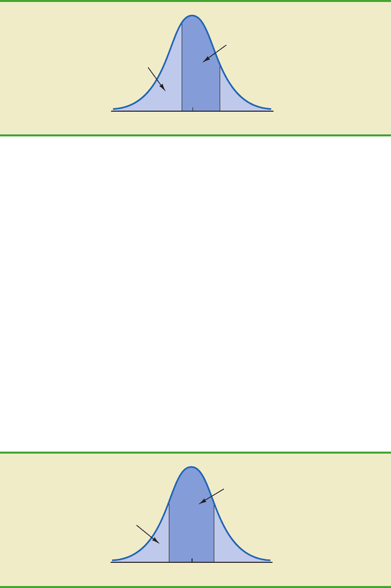
To illustrate the second type of probability calculation, we show how to compute the
probability that z is in the interval between .50 and 1.25; that is, P(.50 z 1.25). The
following graph shows this area, or probability.
01
z
P(z ≤ 1.00)
CH006.qxd 8/16/10 6:34 PM Page 242
Copyright 2010 Cengage Learning. All Rights Reserved. May not be copied, scanned, or duplicated, in whole or in part. Due to electronic rights, some third party content may be suppressed from the eBook and/or eChapter(s).
Editorial review has deemed that any suppressed content does not materially affect the overall learning experience. Cengage Learning reserves the right to remove additional content at any time if subsequent rights restrictions require it.
6.2 Normal Probability Distribution 243
Three steps are required to compute this probability. First, we find the area under the nor-
mal curve to the left of z 1.25. Second, we find the area under the normal curve to the left
of z .50. Finally, we subtract the area to the left of z .50 from the area to the left
of z 1.25 to find P(.50 z 1.25).
To find the area under the normal curve to the left of z 1.25, we first locate the 1.2
row in the standard normal probability table and then move across to the .05 column. Be-
cause the table value in the 1.2 row and the .05 column is .8944, P(z 1.25) .8944. Simi-
larly, to find the area under the curve to the left of z .50, we use the left-hand page of
the table to locate the table value in the .5 row and the .00 column; with a table value of
.3085, P(z .50) .3085. Thus, P(.50 z 1.25) P(z 1.25) P(z .50)
.8944 .3085 .5859.
Let us consider another example of computing the probability that z is in the interval
between two given values. Often it is of interest to compute the probability that a nor-
mal random variable assumes a value within a certain number of standard deviations of
the mean. Suppose we want to compute the probability that the standard normal ran-
dom variable is within one standard deviation of the mean; that is, P(1.00 z 1.00).
To compute this probability we must find the area under the curve between 1.00
and 1.00. Earlier we found that P(z 1.00) .8413. Referring again to the table inside
the front cover of the book, we find that the area under the curve to the left of z 1.00
is .1587, so P(z 1.00) .1587. Therefore, P(1.00 z 1.00) P(z 1.00)
P(z 1.00) .8413 .1587 .6826. This probability is shown graphically in the
following figure.
0 1.00
z
–1.00
P(z ≤ –1.00)
= .1587
P(–1.00 ≤ z ≤ 1.00)
= .8413 – .1587 = .6826
0 1.25–.50
z
P(–.50 ≤ z ≤ 1.25)
P(z < –.50)
CH006.qxd 8/16/10 6:34 PM Page 243
Copyright 2010 Cengage Learning. All Rights Reserved. May not be copied, scanned, or duplicated, in whole or in part. Due to electronic rights, some third party content may be suppressed from the eBook and/or eChapter(s).
Editorial review has deemed that any suppressed content does not materially affect the overall learning experience. Cengage Learning reserves the right to remove additional content at any time if subsequent rights restrictions require it.
244 Chapter 6 Continuous Probability Distributions
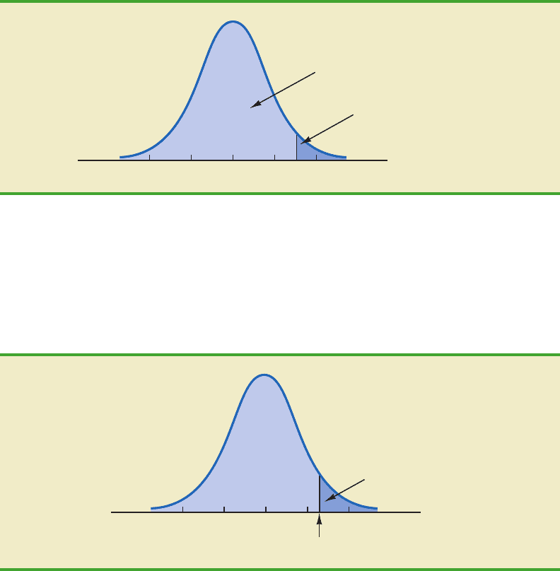
To illustrate how to make the third type of probability computation, suppose we want to
compute the probability of obtaining a zvalue of at least 1.58; that is, P(z 1.58). The value
in the z 1.5 row and the .08 column of the cumulative normal table is .9429; thus, P(z
1.58) .9429. However, because the total area under the normal curve is 1, P(z 1.58)
1 .9429 .0571. This probability is shown in the following figure.
0
z
+1
P(z ≥ 1.58)
= 1.0000 – .9429 = .0571
+2–1–2
P(z < 1.58) = .9429
z
0+1+2–1–2
Probability = .10
What is this z value?
In the preceding illustrations, we showed how to compute probabilities given specified
z values. In some situations, we are given a probability and are interested in working back-
ward to find the corresponding z value. Suppose we want to find a z value such that the
probability of obtaining a larger z value is .10. The following figure shows this situation
graphically.
This problem is the inverse of those in the preceding examples. Previously, we specified
the z value of interest and then found the corresponding probability, or area. In this example,
we are given the probability, or area, and asked to find the corresponding z value. To do so,
we use the standard normal probability table somewhat differently.
Recall that the standard normal probability table gives the area under the curve to the
left of a particular z value. We have been given the information that the area in the upper
tail of the curve is .10. Hence, the area under the curve to the left of the unknown z value
must equal .9000. Scanning the body of the table, we find .8997 is the cumulative proba-
bility value closest to .9000. The section of the table providing this result follows.
Given a probability, we can
use the standard normal
table in an inverse fashion
to find the corresponding z
value.
CH006.qxd 8/16/10 6:34 PM Page 244
Copyright 2010 Cengage Learning. All Rights Reserved. May not be copied, scanned, or duplicated, in whole or in part. Due to electronic rights, some third party content may be suppressed from the eBook and/or eChapter(s).
Editorial review has deemed that any suppressed content does not materially affect the overall learning experience. Cengage Learning reserves the right to remove additional content at any time if subsequent rights restrictions require it.