Anderson D.R., Sweeney D.J., Williams T.A. Essentials of Statistics for Business and Economics
Подождите немного. Документ загружается.


5.3 Expected Value and Variance 205
Applications
17. The number of students taking the SAT has risen to an all-time high of more than 1.5 mil-
lion (College Board, August 26, 2008). Students are allowed to repeat the test in hopes of
improving the score that is sent to college and university admission offices. The number
of times the SAT was taken and the number of students are as follows.
a. Let x be a random variable indicating the number of times a student takes the SAT.
Show the probability distribution for this random variable.
b. What is the probability that a student takes the SAT more than one time?
c. What is the probability that a student takes the SAT three or more times?
d. What is the expected value of the number of times the SAT is taken? What is your in-
terpretation of the expected value?
e. What is the variance and standard deviation for the number of times the SAT is taken?
18. TheAmerican Housing Survey reported the following data on the number of bedrooms in
owner-occupiedand renter-occupied houses in centralcities (U.S. Census Bureau website,
March 31, 2003).
a. Define a random variable x ⫽ number of bedrooms in renter-occupied houses and
develop a probability distribution for the random variable. (Let x ⫽ 4 represent 4 or
more bedrooms.)
b. Compute the expected value and variance for the number of bedrooms in renter-
occupied houses.
c. Define a random variable y ⫽ number of bedrooms in owner-occupied houses and
develop a probability distribution for the random variable. (Let y ⫽ 4 represent 4 or
more bedrooms.)
d. Compute the expected value and variance for the number of bedrooms in owner-
occupied houses.
e. What observations can you make from a comparison of the number of bedrooms in
renter-occupied versus owner-occupied homes?
19. The National Basketball Association (NBA) records a variety of statistics for each team.
Two of these statistics are the percentage of field goals made by the team and the percent-
age of three-point shots made by the team. For a portion of the 2004 season, the shooting
records of the 29 teams in the NBA showed that the probability of scoring two points by
test
SELF
Number of Houses (1000s)
Bedrooms Renter-Occupied Owner-Occupied
0 547 23
1 5012 541
2 6100 3832
3 2644 8690
4 or
more 557 3783
Number of Number of
Times Students
1 721,769
2 601,325
3 166,736
4 22,299
5 6,730
CH005.qxd 8/16/10 6:31 PM Page 205
Copyright 2010 Cengage Learning. All Rights Reserved. May not be copied, scanned, or duplicated, in whole or in part. Due to electronic rights, some third party content may be suppressed from the eBook and/or eChapter(s).
Editorial review has deemed that any suppressed content does not materially affect the overall learning experience. Cengage Learning reserves the right to remove additional content at any time if subsequent rights restrictions require it.

206 Chapter 5 Discrete Probability Distributions
making a field goal was .44, and the probability of scoring three points by making a three-
point shot was .34 (NBA website, January 3, 2004).
a. What is the expected value of a two-point shot for these teams?
b. What is the expected value of a three-point shot for these teams?
c. If the probability of making a two-point shot is greater than the probability of making
a three-point shot, why do coaches allow some players to shoot the three-point shot if
they have the opportunity? Use expected value to explain your answer.
20. The probability distribution for damage claims paid by the Newton Automobile Insurance
Company on collision insurance follows.
a. Use the expected collision payment to determine the collision insurance premium that
would enable the company to break even.
b. The insurance company charges an annual rate of $520 for the collision coverage.
What is the expected value of the collision policy for a policyholder? (Hint: It is the
expected payments from the company minus the cost of coverage.) Why does the
policyholder purchase a collision policy with this expected value?
21. The following probability distributions of job satisfaction scores for a sample of information
systems (
IS) senior executives and middle managers range from a low of 1 (very dissatisfied)
to a high of 5 (very satisfied).
Payment ($) Probability
0 .85
500 .04
1000 .04
3000 .03
5000 .02
8000 .01
10000 .01
Probability
Job Satisfaction IS Senior IS Middle
Score Executives Managers
1 .05 .04
2 .09 .10
3 .03 .12
4 .42 .46
5 .41 .28
a. What is the expected value of the job satisfaction score for senior executives?
b. What is the expected value of the job satisfaction score for middle managers?
c. Compute the variance of job satisfaction scores for executives and middle managers.
d. Compute the standard deviation of job satisfaction scores for both probability distributions.
e. Compare the overall job satisfaction of senior executives and middle managers.
22. The demand for a product of Carolina Industries varies greatly from month to month. The
probability distribution in the following table, based on the past two years of data, shows
the company’s monthly demand.
Unit Demand Probability
300 .20
400 .30
500 .35
600 .15
CH005.qxd 8/16/10 6:31 PM Page 206
Copyright 2010 Cengage Learning. All Rights Reserved. May not be copied, scanned, or duplicated, in whole or in part. Due to electronic rights, some third party content may be suppressed from the eBook and/or eChapter(s).
Editorial review has deemed that any suppressed content does not materially affect the overall learning experience. Cengage Learning reserves the right to remove additional content at any time if subsequent rights restrictions require it.

5.4 Binomial Probability Distribution 207
a. If the company bases monthly orders on the expected value of the monthly demand,
what should Carolina’s monthly order quantity be for this product?
b. Assume that each unit demanded generates $70 in revenue and that each unit ordered
costs $50. How much will the company gain or lose in a month if it places an order
based on your answer to part (a) and the actual demand for the item is 300 units?
23. The New York City Housing and Vacancy Survey showed a total of 59,324 rent-controlled
housing units and 236,263 rent-stabilized units built in 1947 or later. For these rental units,
the probability distributions for the number of persons living in the unit are given
(U.S. Census Bureau website, January 12, 2004).
a. What is the expected value of the number of persons living in each type of unit?
b. What is the variance of the number of persons living in each type of unit?
c. Make some comparisons between the number of persons living in rent-controlled units
and the number of persons living in rent-stabilized units.
24. The J. R. Ryland Computer Company is considering a plant expansion to enable the com-
pany to begin production of a new computer product. The company’s president must deter-
mine whether to make the expansion a medium- or large-scale project. Demand for the new
product is uncertain, which for planning purposes may be low demand, medium demand, or
high demand. The probability estimates for demand are .20, .50, and .30, respectively. Let-
ting x and y indicate the annual profit in thousands of dollars, the firm’s planners developed
the following profit forecasts for the medium- and large-scale expansion projects.
a. Compute the expected value for the profit associated with the two expansion alterna-
tives. Which decision is preferred for the objective of maximizing the expected profit?
b. Compute the variance for the profit associated with the two expansion alternatives.
Which decision is preferred for the objective of minimizing the risk or uncertainty?
5.4 Binomial Probability Distribution
The binomial probability distribution is a discrete probability distribution that provides
many applications. It is associated with a multiple-step experiment that we call the bino-
mial experiment.
Number of
Persons Rent-Controlled Rent-Stabilized
1 .61 .41
2 .27 .30
3 .07 .14
4 .04 .11
5 .01 .03
6 .00 .01
Medium-Scale Large-Scale
Expansion Profit Expansion Profit
xf(x) yf(y)
Low 50
.20 0 .20
Demand Medium 150 .50 100 .50
High 200 .30 300 .30
CH005.qxd 8/16/10 6:31 PM Page 207
Copyright 2010 Cengage Learning. All Rights Reserved. May not be copied, scanned, or duplicated, in whole or in part. Due to electronic rights, some third party content may be suppressed from the eBook and/or eChapter(s).
Editorial review has deemed that any suppressed content does not materially affect the overall learning experience. Cengage Learning reserves the right to remove additional content at any time if subsequent rights restrictions require it.

208 Chapter 5 Discrete Probability Distributions
A Binomial Experiment
A binomial experiment exhibits the following four properties.
If properties 2, 3, and 4 are present, we say the trials are generated by a Bernoulli process.
If, in addition, property 1 is present, we say we have a binomial experiment. Figure 5.2 de-
picts one possible sequence of successes and failures for a binomial experiment involving
eight trials.
In a binomial experiment, our interest is in the number of successes occurring in the n
trials. If we let x denote the number of successes occurring in the n trials, we see that x can
assume the values of 0, 1, 2, 3,..., n. Because the number of values is finite, x is a discrete
random variable. The probability distribution associated with this random variable is called
the binomial probability distribution. For example, consider the experiment of tossing a
coin five times and on each toss observing whether the coin lands with a head or a tail on
its upward face. Suppose we want to count the number of heads appearing over the five
tosses. Does this experiment show the properties of a binomial experiment? What is the ran-
dom variable of interest? Note that
1. The experiment consists of five identical trials; each trial involves the tossing of
one coin.
2. Two outcomes are possible for each trial: a head or a tail. We can designate head a
success and tail a failure.
3. The probability of a head and the probability of a tail are the same for each trial,
with p ⫽ .5 and 1 ⫺ p ⫽ .5.
4. The trials or tosses are independent because the outcome on any one trial is not
affected by what happens on other trials or tosses.
PROPERTIES OF A BINOMIAL EXPERIMENT
1. The experiment consists of a sequence of n identical trials.
2. Two outcomes are possible on each trial. We refer to one outcome as a suc-
cess and the other outcome as a failure.
3. The probability of a success, denoted by p, does not change from trial to trial.
Consequently, the probability of a failure, denoted by 1 ⫺ p, does not change
from trial to trial.
4. The trials are independent.
Property 1: The experiment consists of
n 8 identical trials.
Property 2: Each trial results in either
success (S) or failure (F).
Trials 12345678
Outcomes S FFSSF SS
FIGURE 5.2 ONE POSSIBLE SEQUENCE OF SUCCESSES AND FAILURES
FOR AN EIGHT-TRIAL BINOMIAL EXPERIMENT
Jakob Bernoulli
(1654–1705), the first of the
Bernoulli family of Swiss
mathematicians, published
a treatise on probability
that contained the theory
of permutations and
combinations, as well as
the binomial theorem.
CH005.qxd 8/16/10 6:31 PM Page 208
Copyright 2010 Cengage Learning. All Rights Reserved. May not be copied, scanned, or duplicated, in whole or in part. Due to electronic rights, some third party content may be suppressed from the eBook and/or eChapter(s).
Editorial review has deemed that any suppressed content does not materially affect the overall learning experience. Cengage Learning reserves the right to remove additional content at any time if subsequent rights restrictions require it.
5.4 Binomial Probability Distribution 209
Thus, the properties of a binomial experiment are satisfied. The random variable of inter-
est is x ⫽ the number of heads appearing in the five trials. In this case, x can assume the
values of 0, 1, 2, 3, 4, or 5.
As another example, consider an insurance salesperson who visits 10 randomly selected
families. The outcome associated with each visit is classified as a success if the family pur-
chases an insurance policy and a failure if the family does not. From past experience, the
salesperson knows the probability that a randomly selected family will purchase an insur-
ance policy is .10. Checking the properties of a binomial experiment, we observe that
1. The experiment consists of 10 identical trials; each trial involves contacting one family.
2. Two outcomes are possible on each trial: the family purchases a policy (success) or
the family does not purchase a policy (failure).
3. The probabilities of a purchase and a nonpurchase are assumed to be the same for
each sales call, with p ⫽ .10 and 1 ⫺ p ⫽ .90.
4. The trials are independent because the families are randomly selected.
Because the four assumptions are satisfied, this example is a binomial experiment. The
random variable of interest is the number of sales obtained in contacting the 10 families. In
this case, x can assume the values of 0, 1, 2, 3, 4, 5, 6, 7, 8, 9, and 10.
Property 3 of the binomial experiment is called the stationarity assumption and is
sometimes confused with property 4, independence of trials. To see how they differ, consider
again the case of the salesperson calling on families to sell insurance policies. If, as the day
wore on, the salesperson got tired and lost enthusiasm, the probability of success (selling a
policy) might drop to .05, for example, by the tenth call. In such a case, property 3 (station-
arity) would not be satisfied, and we would not have a binomial experiment. Even if prop-
erty 4 held—that is, the purchase decisions of each family were made independently—it
would not be a binomial experiment if property 3 was not satisfied.
In applications involving binomial experiments, a special mathematical formula, called
the binomial probability function, can be used to compute the probability of x successes
in the n trials. Using probability concepts introduced in Chapter 4, we will show in the
context of an illustrative problem how the formula can be developed.
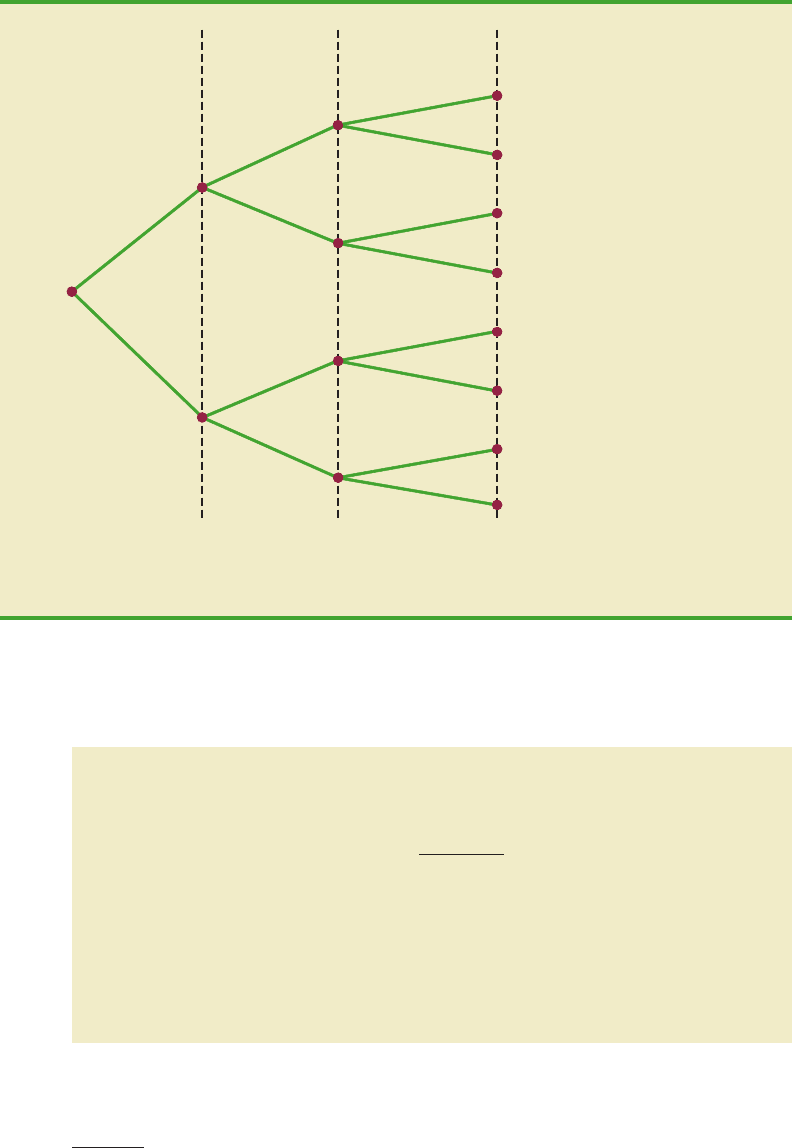
Martin Clothing Store Problem
Let us consider the purchase decisions of the next three customers who enter the Martin
Clothing Store. On the basis of past experience, the store manager estimates the probability
that any one customer will make a purchase is .30. What is the probability that two of the
next three customers will make a purchase?
Using a tree diagram (Figure 5.3), we can see that the experiment of observing the three
customers each making a purchase decision has eight possible outcomes. Using S to denote
success (a purchase) and F to denote failure (no purchase), we are interested in experi-
mental outcomes involving two successes in the three trials (purchase decisions). Next, let
us verify that the experiment involving the sequence of three purchase decisions can be
viewed as a binomial experiment. Checking the four requirements for a binomial experi-
ment, we note that:
1. The experiment can be described as a sequence of three identical trials, one trial for
each of the three customers who will enter the store.
2. Two outcomes—the customer makes a purchase (success) or the customer does not
make a purchase (failure)—are possible for each trial.
3. The probability that the customer will make a purchase (.30) or will not make a pur-
chase (.70) is assumed to be the same for all customers.
4. The purchase decision of each customer is independent of the decisions of the
other customers.
CH005.qxd 8/16/10 6:31 PM Page 209
Copyright 2010 Cengage Learning. All Rights Reserved. May not be copied, scanned, or duplicated, in whole or in part. Due to electronic rights, some third party content may be suppressed from the eBook and/or eChapter(s).
Editorial review has deemed that any suppressed content does not materially affect the overall learning experience. Cengage Learning reserves the right to remove additional content at any time if subsequent rights restrictions require it.
210 Chapter 5 Discrete Probability Distributions
Hence, the properties of a binomial experiment are present.
The number of experimental outcomes resulting in exactly x successes in n trials can
be computed using the following formula.
1
Third
Customer
Experimental
Outcome
S
(S, S, S)
F
3
Value of x
(S, S, F)2
S
(S, F, S)
F
2
(S, F, F)1
S
(F, S, S)
F
2
(F, S, F)1
S
(F, F, S)
F
1
(F, F, F)0
S
F
S
F
S
F
Second
Customer
First
Customer
S Purchase
F No purchase
x Number of customers makin
g
a purchase
FIGURE 5.3 TREE DIAGRAM FOR THE MARTIN CLOTHING STORE PROBLEM
NUMBER OF EXPERIMENTAL OUTCOMES PROVIDING EXACTLY x
SUCCESSES IN n TRIALS
(5.6)
where
and, by definition,
0! ⫽ 1
n! ⫽ n(n ⫺ 1)(n ⫺ 2)
. . .
(2)(1)
冢
n
x
冣
⫽
n!
x!(n ⫺ x)!
Now let us return to the Martin Clothing Store experiment involving three customer
purchase decisions. Equation (5.6) can be used to determine the number of experimental
1
This formula, introduced in Chapter 4, determines the number of combinations of n objects selected x at a time. For the bi-
nomial experiment, this combinatorial formula provides the number of experimental outcomes (sequences of n trials) result-
ing in x successes.
CH005.qxd 8/16/10 6:31 PM Page 210
Copyright 2010 Cengage Learning. All Rights Reserved. May not be copied, scanned, or duplicated, in whole or in part. Due to electronic rights, some third party content may be suppressed from the eBook and/or eChapter(s).
Editorial review has deemed that any suppressed content does not materially affect the overall learning experience. Cengage Learning reserves the right to remove additional content at any time if subsequent rights restrictions require it.

5.4 Binomial Probability Distribution 211
outcomes involving two purchases; that is, the number of ways of obtaining x ⫽ 2 successes
in the n ⫽ 3 trials. From equation (5.6) we have
Equation (5.6) shows that three of the experimental outcomes yield two successes. From
Figure 5.3 we see that these three outcomes are denoted by (S, S, F), (S, F, S), and (F, S, S).
Using equation (5.6) to determine how many experimental outcomes have three
successes (purchases) in the three trials, we obtain
From Figure 5.3 we see that the one experimental outcome with three successes is identi-
fied by (S, S, S).
We know that equation (5.6) can be used to determine the number of experimental out-
comes that result in x successes. If we are to determine the probability of x successes in
n trials, however, we must also know the probability associated with each of these experi-
mental outcomes. Because the trials of a binomial experiment are independent, we can sim-
ply multiply the probabilities associated with each trial outcome to find the probability of
a particular sequence of successes and failures.
The probability of purchases by the first two customers and no purchase by the third
customer, denoted (S, S, F), is given by
With a .30 probability of a purchase on any one trial, the probability of a purchase on the
first two trials and no purchase on the third is given by
Two other experimental outcomes also result in two successes and one failure. The proba-
bilities for all three experimental outcomes involving two successes follow.
(.30)(.30)(.70) ⫽ (.30)
2
(.70) ⫽ .063
pp(1 ⫺ p)
冢
n
x
冣
⫽
冢
3
3
冣
⫽
3!
3!(3 ⫺ 3)!
⫽
3!
3!0!
⫽
(3)(2)(1)
3(2)(1)(1)
⫽
6
6
⫽ 1
冢
n
x
冣
⫽
冢
3
2
冣
⫽
3!
2!(3 ⫺ 2)!
⫽
(3)(2)(1)
(2)(1)(1)
⫽
6
2
⫽ 3
Trial Outcomes
Probability of
1st 2nd 3rd Experimental Experimental
Customer Customer Customer Outcome Outcome
Purchase Purchase No purchase (S, S, F) pp(1 ⫺ p) ⫽ p
2
(1 ⫺ p)
⫽ (.30)
2
(.70) ⫽ .063
Purchase No purchase Purchase (S, F, S) p(1 ⫺ p)p ⫽ p
2
(1 ⫺ p)
⫽ (.30)
2
(.70) ⫽ .063
No purchase Purchase Purchase (F, S, S)(1⫺ p)pp ⫽ p
2
(1 ⫺ p)
⫽ (.30)
2
(.70) ⫽ .063
Observe that all three experimental outcomes with two successes have exactly the same
probability. This observation holds in general. In any binomial experiment, all sequences
of trial outcomes yielding x successes in n trials have the same probability of occurrence.
The probability of each sequence of trials yielding x successes in n trials follows.
CH005.qxd 8/16/10 6:31 PM Page 211
Copyright 2010 Cengage Learning. All Rights Reserved. May not be copied, scanned, or duplicated, in whole or in part. Due to electronic rights, some third party content may be suppressed from the eBook and/or eChapter(s).
Editorial review has deemed that any suppressed content does not materially affect the overall learning experience. Cengage Learning reserves the right to remove additional content at any time if subsequent rights restrictions require it.

212 Chapter 5 Discrete Probability Distributions
(5.7)
For the Martin Clothing Store, this formula shows that any experimental outcome with two
successes has a probability of p
2
(1 ⫺ p)
(3⫺2)
⫽ p
2
(1 ⫺ p)
1
⫽ (.30)
2
(.70)
1
⫽ .063.
Because equation (5.6) shows the number of outcomes in a binomial experiment with x
successes and equation (5.7) gives the probability for each sequence involving x successes,
we combine equations (5.6) and (5.7) to obtain the following binomial probability function.
Probability of a particular
sequence of trial outcomes
with x successes in n trials
⫽ p
x
(1 ⫺ p)
(n⫺x)
For the binomial probability distribution, x is a discrete random variable with the probabil-
ity function f(x) applicable for values of x ⫽ 0, 1, 2,...,n.
In the Martin Clothing Store example, let us use equation (5.8) to compute the proba-
bility that no customer makes a purchase, exactly one customer makes a purchase, exactly
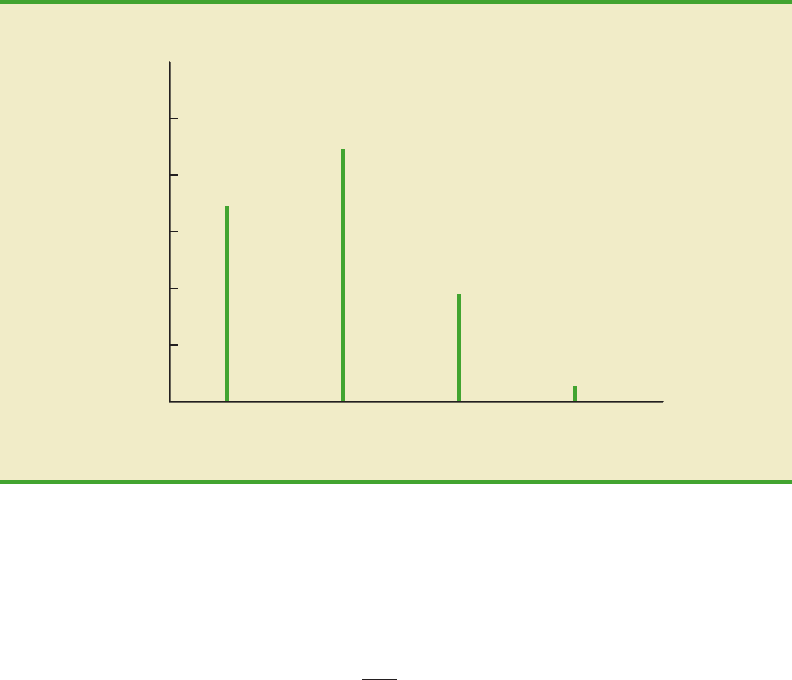
two customers make a purchase, and all three customers make a purchase. The calculations
are summarized in Table 5.6, which gives the probability distribution of the number of cus-
tomers making a purchase. Figure 5.4 is a graph of this probability distribution.
The binomial probability function can be applied to any binomial experiment. If we are
satisfied that a situation demonstrates the properties of a binomial experiment and if we
know the values of n and p, we can use equation (5.8) to compute the probability of x suc-
cesses in the n trials.
BINOMIAL PROBABILITY FUNCTION
(5.8)
where
x ⫽
p ⫽
n ⫽
f(x) ⫽
冢
n
x
冣
⫽
the number of successes
the probability of a success on one trial
the number of trials
the probability of x successes in n trials
n!
x!(n ⫺ x)!
f(x) ⫽
冢
n
x
冣
p
x
(1 ⫺ p)
(n⫺x)
xf(x)
0 (.30)
0
(.70)
3
⫽ .343
1 (.30)
1
(.70)
2
⫽ .441
2 (.30)
2
(.70)
1
⫽ .189
3 (.30)
3
(.70)
0
⫽ .027
1.000
3!
3!0!
3!
2!1!
3!
1!2!
3!
0!3!
TABLE 5.6
PROBABILITY DISTRIBUTION FOR THE NUMBER OF CUSTOMERS
MAKING A PURCHASE
CH005.qxd 8/16/10 6:31 PM Page 212
Copyright 2010 Cengage Learning. All Rights Reserved. May not be copied, scanned, or duplicated, in whole or in part. Due to electronic rights, some third party content may be suppressed from the eBook and/or eChapter(s).
Editorial review has deemed that any suppressed content does not materially affect the overall learning experience. Cengage Learning reserves the right to remove additional content at any time if subsequent rights restrictions require it.
5.4 Binomial Probability Distribution 213
If we consider variations of the Martin experiment, such as 10 customers rather than 3
entering the store, the binomial probability function given by equation (5.8) is still applic-
able. Suppose we have a binomial experiment with n ⫽ 10, x ⫽ 4, and p ⫽ .30. The prob-
ability of making exactly four sales to 10 customers entering the store is
Using Tables of Binomial Probabilities
Tables have been developed that give the probability of x successes in n trials for a binomial
experiment. The tables are generally easy to use and quicker than equation (5.8). Table 5 of
Appendix B provides such a table of binomial probabilities. Aportion of this table appears
in Table 5.7. To use this table, we must specify the values of n, p, and x for the binomial ex-
periment of interest. In the example at the top of Table 5.7, we see that the probability of
x ⫽ 3 successes in a binomial experiment with n ⫽ 10 and p ⫽ .40 is .2150. You can use
equation (5.8) to verify that you would obtain the same answer if you used the binomial
probability function directly.
Now let us use Table 5.7 to verify the probability of four successes in 10 trials for the
Martin Clothing Store problem. Note that the value of f(4) ⫽ .2001 can be read directly
from the table of binomial probabilities, with n ⫽ 10, x ⫽ 4, and p ⫽ .30.
Even though the tables of binomial probabilities are relatively easy to use, it is im-
possible to have tables that show all possible values of n and p that might be encountered
in a binomial experiment. However, with today’s calculators, using equation (5.8) to
calculate the desired probability is not difficult, especially if the number of trials is not
large. In the exercises, you should practice using equation (5.8) to compute the binomial
probabilities unless the problem specifically requests that you use the binomial proba-
bility table.
f(4) ⫽
10!
4!6!
(.30)
4
(.70)
6
⫽ .2001
.40
.30
.20
.10
.00
f (x)
Probability
Number of Customers Making a Purchase
0 1 2
x
3
.50
FIGURE 5.4 GRAPHICAL REPRESENTATION OF THE PROBABILITY DISTRIBUTION
FOR THE NUMBER OF CUSTOMERS MAKING A PURCHASE
With modern calculators,
these tables are almost
unnecessary. It is easy to
evaluate equation (5.8)
directly.
CH005.qxd 8/16/10 6:31 PM Page 213
Copyright 2010 Cengage Learning. All Rights Reserved. May not be copied, scanned, or duplicated, in whole or in part. Due to electronic rights, some third party content may be suppressed from the eBook and/or eChapter(s).
Editorial review has deemed that any suppressed content does not materially affect the overall learning experience. Cengage Learning reserves the right to remove additional content at any time if subsequent rights restrictions require it.

214 Chapter 5 Discrete Probability Distributions
Statistical software packages such as Minitab and spreadsheet packages such as Excel
also provide a capability for computing binomial probabilities. Consider the Martin Cloth-
ing Store example with n ⫽ 10 and p ⫽ .30. Figure 5.5 shows the binomial probabilities
generated by Minitab for all possible values of x. Note that these values are the same as
those found in the p ⫽ .30 column of Table 5.7. Appendix 5.1 gives the step-by-step pro-
cedure for using Minitab to generate the output in Figure 5.5. Appendix 5.2 describes how
Excel can be used to compute binomial probabilities.
Expected Value and Variance for the
Binomial Distribution
In Section 5.3 we provided formulas for computing the expected value and variance
of a discrete random variable. In the special case where the random variable has a bi-
nomial distribution with a known number of trials n and a known probability of success p,
the general formulas for the expected value and variance can be simplified. The results
follow.
p
nx.05 .10 .15 .20 .25 .30 .35 .40 .45 .50
9 0 .6302 .3874 .2316 .1342 .0751 .0404 .0207 .0101 .0046 .0020
1 .2985 .3874 .3679 .3020 .2253 .1556 .1004 .0605 .0339 .0176
2 .0629 .1722 .2597 .3020 .3003 .2668 .2162 .1612 .1110 .0703
3 .0077 .0446 .1069 .1762 .2336 .2668 .2716 .2508 .2119 .1641
4 .0006 .0074 .0283 .0661 .1168 .1715 .2194 .2508 .2600 .2461
5 .0000 .0008 .0050 .0165 .0389 .0735 .1181 .1672 .2128 .2461
6 .0000 .0001 .0006 .0028 .0087 .0210 .0424 .0743 .1160 .1641
7 .0000 .0000 .0000 .0003 .0012 .0039 .0098 .0212 .0407 .0703
8 .0000 .0000 .0000 .0000 .0001 .0004 .0013 .0035 .0083 .0176
9 .0000 .0000 .0000 .0000 .0000 .0000 .0001 .0003 .0008 .0020
10 0 .5987 .3487 .1969 .1074 .0563 .0282 .0135 .0060 .0025 .0010
1 .3151 .3874 .3474 .2684 .1877 .1211 .0725 .0403 .0207 .0098
2 .0746 .1937 .2759 .3020 .2816 .2335 .1757 .1209 .0763 .0439
3 .0105 .0574 .1298 .2013 .2503 .2668 .2522 .2150 .1665 .1172
4 .0010 .0112 .0401 .0881 .1460 .2001 .2377 .2508 .2384 .2051
5 .0001 .0015 .0085 .0264 .0584 .1029 .1536 .2007 .2340 .2461
6 .0000 .0001 .0012 .0055 .0162 .0368 .0689 .1115 .1596 .2051
7 .0000 .0000 .0001 .0008 .0031 .0090 .0212 .0425 .0746 .1172
8 .0000 .0000 .0000 .0001 .0004 .0014 .0043 .0106 .0229 .0439
9 .0000 .0000 .0000 .0000 .0000 .0001 .0005 .0016 .0042 .0098
10 .0000 .0000 .0000 .0000 .0000 .0000 .0000 .0001 .0003 .0010
TABLE 5.7
SELECTED VALUES FROM THE BINOMIAL PROBABILITYTABLE
EXAMPLE: n ⫽ 10, x ⫽ 3, p ⫽ .40; f(3) ⫽ .2150
EXPECTED VALUE AND VARIANCE FOR THE BINOMIAL DISTRIBUTION
(5.9)
(5.10)
Var(x) ⫽ σ
2
⫽ np(1 ⫺ p)
E(x) ⫽ μ ⫽ np
CH005.qxd 8/16/10 6:31 PM Page 214
Copyright 2010 Cengage Learning. All Rights Reserved. May not be copied, scanned, or duplicated, in whole or in part. Due to electronic rights, some third party content may be suppressed from the eBook and/or eChapter(s).
Editorial review has deemed that any suppressed content does not materially affect the overall learning experience. Cengage Learning reserves the right to remove additional content at any time if subsequent rights restrictions require it.