Articolo G.A. Partial Differential Equations and Boundary Value Problems with Maple V
Подождите немного. Документ загружается.


498 Chapter 8
> T1(t):=exp(−k*lambda[n]*t);
T 1(t) := e
−
1
4
n
2
π
2
t
(8.34)
First-order Green’s function
> G1(t,tau):=simplify(T1(t)/(subs(t=tau,T1(t))));
G1(t, τ) := e
−
1
4
π
2
n
2
(t−τ)
(8.35)
Time-dependent solution
> T[n](t):=eval(C(n)*T1(t)+Int(G1(t,tau)*Q[n](tau),tau=0..t)):T[n](t):=value(%);
T
n
(t) := C(n)e
−
1
4
n
2
π
2
t
−
4
√
2
−n
2
π
2
e
−
1
4
n
2
π
2
t
+n
2
π
2
cos(t) +4 sin(t)
nπ
n
4
π
4
+16
(8.36)
Generalized series terms
> v[n](x,t):=(eval(T[n](t)*X[n](x))):
Variable portion of solution
> v(x,t):=Sum(v[n](x,t),n=1..infinity);
v(x, t) :=
∞
n=1
⎛
⎜
⎜
⎝
C(n)e
−
1
4
n
2
π
2
t
−
4
√
2
−n
2
π
2
e
−
1
4
n
2
π
2
t
+n
2
π
2
cos(t) +4 sin(t)
nπ
n
4
π
4
+16
⎞
⎟
⎟
⎠
√
2 sin(nπx)
(8.37)
The Fourier coefficients C(n) are determined from the integral in Section 8.3 for the special
case where
> f(x):=x*(1−x);
f(x) := x(1 −x) (8.38)
> C(n):=Int((f(x)−s(x,0))*X[n](x),x=0..a);C(n):=expand(value(%)):
C(n) :=
1
0
x(1 −x)
√
2 sin(nπx) dx (8.39)
> C(n):=simplify(subs({sin(n*Pi)=0,cos(n*Pi)=(−1)ˆn},C(n)));
C(n) := −
2
√
2
−1 +(−1)
n
π
3
n
3
(8.40)
for n = 1, 2, 3,....

Nonhomogeneous Partial Differential Equations 499
> T[n](t):=(C(n)*T1(t)+int(G1(t,tau)*Q[n](tau),tau=0..t));
T
n
(t) := −
2
√
2
−1 +(−1)
n
e
−
1
4
n
2
π
2
t
π
3
n
3
−
4
√
2
−n
2
π
2
e
−
1
4
n
2
π
2
t
+n
2
π
2
cos(t) +4 sin(t)
πn
n
4
π
4
+16
(8.41)
Generalized series terms
> v[n](x,t):=(T[n](t)*X[n](x));
v
n
(x, t) :=
⎛
⎝
−
2
√
2
−1 +(−1)
n
e
−
1
4
n
2
π
2
t
π
3
n
3
−
4
√
2
−n
2
π
2
e
−
1
4
n
2
π
2
t
+n
2
π
2
cos(t) +4 sin(t)
πn
n
4
π
4
+16
⎞
⎟
⎟
⎠
√
2 sin(nπx)
(8.42)
Final solution (linear plus variable portion)
> u(x,t):=(eval(Sum(v[n](x,t),n=1..infinity)+s(x,t)));
u(x, t) :=
∞
n=1
⎛
⎝
−
2
√
2
−1 +(−1)
n
e
−
1
4
n
2
π
2
t
π
3
n
3
(8.43)
−
4
√
2
−n
2
π
2
e
−
1
4
n
2
π
2
t
−n
2
π
2
cos(t) −4 sin(t)
πn
n
4
π
4
+16
⎞
⎟
⎟
⎠
√
2 sin(nπx) −sin(t)x +sin(t)
First few terms of sum
> u(x,t):=s(x,t)+sum(v[n](x,t),n=1..3):
ANIMATION
> animate(u(x,t),x=0..a,t=0..5,thickness=3);
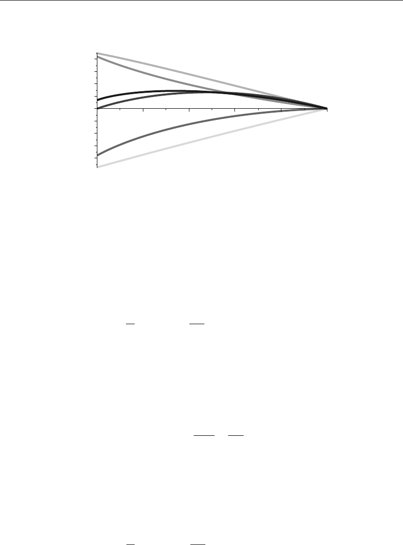
The preceding animation command displays the spatial-time-dependent solution of u(x, t) for
the given boundary conditions and initial conditions. The animation sequence here and in
Figure 8.2 shows snapshots of the animation at times t = 0, 1, 2, 3, 4, 5. Note how the solution
satisfies the given boundary and initial conditions.
ANIMATION SEQUENCE
> u(x,0):=subs(t=0,u(x,t)):u(x,1):=subs(t=1,u(x,t)):
> u(x,2):=subs(t=2,u(x,t)):u(x,3):=subs(t=3,u(x,t)):
500 Chapter 8
> u(x,4):=subs(t=4,u(x,t)):u(x,5):=subs(t=5,u(x,t)):
> plot({u(x,0),u(x,1),u(x,2),u(x,3),u(x,4),u(x,5)},x=0..a,thickness=10);
0.8
20.8
0.2 0.4 0.6 0.8 1
0.6
20.6
0.4
20.4
0.2
20.2
0
x
Figure 8.2
EXAMPLE 8.4.3: We seek the temperature distribution u(x, t) in a thin rod whose lateral
surface is insulated over the interval I ={x |0 <x<1}. The left end of the rod is held at a
fixed temperature of 5, and the right end loses heat by convection into a medium whose
temperature is 10. In addition, there is an internal heat source term h(x, t) that increases
linearly with time. The thermal diffusivity of the rod is k = 1/20, and an initial temperature
distribution u(x, 0) = f(x) is given as follows.
SOLUTION: The nonhomogeneous diffusion equation is
∂
∂t
u(x, t) = k
∂
2
∂x
2
u(x, t)
+h(x, t)
The boundary conditions are nonhomogeneous type 1 at the left and nonhomogeneous type 3
at the right:
u(0,t)= 5 and u(1,t)+u
x
(1,t)= 10
The initial condition is
u(x, 0) =−
40x
2
3
+
45x
2
+5
The internal heat source term is
h(x, t) = t
The solution is u(x, t) = v(x, t) +s(x, t), where s(x, t) is the linear portion of the solution and
v(x, t) is the variable portion of the solution, which satisfies the partial differential equation
∂
∂t
v(x, t) = k
∂
2
∂x
2
v(x, t)
+q(x, t)

Nonhomogeneous Partial Differential Equations 501
where
q(x, t) = h(x, t) −
∂
∂t
s(x, t)
Assignment of system parameters
> restart: with(plots):a:=1:k:=1/20:h(x,t):=t:
> A(t):=5:B(t):=10:kappa[1]:=1:kappa[2]:=0:kappa[3]:=1:kappa[4]:=1:
> b(t):=(kappa[3]*a*A(t)+A(t)*kappa[4]−B(t)*kappa[2])/(kappa[1]*kappa[3]*a+kappa[1]*
kappa[4]−kappa[2]*kappa[3]);
b(t) := 5 (8.44)
> m(t):=(kappa[1]*B(t)−A(t)*kappa[3])/(kappa[1]*kappa[3]*a+kappa[1]*
kappa[4]−kappa[2]*kappa[3]);
m(t) :=
5
2
(8.45)
Linear portion of solution
> s(x,t):=m(t)*x+b(t);s(x,0):=eval(subs(t=0,s(x,t))):
s(x, t) :=
5
2
x +5 (8.46)
By the method of separation of variables, the variable solution is
v(x, t) =
∞
n=0
X
n
(x)T
n
(t)
where T
n
(t) is the solution to the time-dependent differential equation
d
dt
T
n
(t) +kλ
n
T
n
(t) = Q
n
(t)
and X
n
(x) is the solution to the spatial-dependent eigenvalue equation
d
2
dx
2
X
n
(x) +λ
n
X
n
(x) = 0
with boundary conditions
X(0) = 0 and X(1) +X
x
(1,t)= 0
The corresponding homogeneous eigenfunction problem consists of the Euler equation, along
with the homogeneous boundary conditions that are type 1 at the left and type 3 at the right.

502 Chapter 8
The allowed eigenvalues and corresponding orthonormal eigenfunctions are obtained from
Example 2.5.4. The eigenvalues λ
n
are the roots of the eigenvalue equation
> tan(sqrt(lambda[n]*a))=−sqrt(lambda[n]);
tan
λ
n
=−
λ
n
(8.47)
> X[n](x):=sqrt(2)*sin(sqrt(lambda[n])*x)/sqrt((cos(sqrt(lambda[n])*a)ˆ2+a));X[m](x):=
subs(n=m,X[n](x)):
X
n
(x) :=
√
2 sin
√
λ
n
x
cos
√
λ
n
2
+1
(8.48)
for n = 1, 2, 3,....
Statement of orthonormality with the respective weight function w(x) = 1
> w(x):=1:Int(X[n](x)*X[m](x),x=0..a)=delta(n,m);
1
0
2 sin
√
λ
n
x
sin
√
λ
m
x
cos
√
λ
n
2
+1
cos
√
λ
m
2
+1
dx = δ(n, m) (8.49)
Time-dependent equation
> diff(T[n](t),t)+k*lambda[n]*T[n](t)=Q[n](t);
d
dt
T
n
(t) +
1
20
λ
n
T
n
(t) = Q
n
(t) (8.50)
> q(x,t):=h(x,t)−diff(s(x,t),t);
q(x, t) := t (8.51)
> Q[n](t):=Int(q(x,t)*X[n](x),x=0..a);Q[n](t):=expand(value(%)):
Q
n
(t) :=
1
0
t
√
2 sin
√
λ
n
x
cos
√
λ
n
2
+1
dx (8.52)
> Q[n](t):=simplify(factor(subs({sin(n*Pi)=0,cos(n*Pi)=(−1)ˆn},Q[n](t))));
Q[n](tau):=subs(t=tau,%):
Q
n
(t) := −
t
√
2
−1 +cos
√
λ
n
cos
√
λ
n
2
+1
√
λ
n
(8.53)

Nonhomogeneous Partial Differential Equations 503
Basis vector
> T1(t):=exp(−k*lambda[n]*t);
T 1(t) := e
−
1
20
λ
n
t
(8.54)
First-order Green’s function
> G1(t,tau):=simplify(T1(t)/(subs(t=tau,T1(t))));
G1(t, τ) := e
−
1
20
λ
n
(t−τ)
(8.55)
Time-dependent solution
> T[n](t):=eval(C(n)*T1(t)+Int(G1(t,tau)*Q[n](tau),tau=0..t));
T
n
(t) := C(n)e
−
1
20
λ
n
t
+
t
0
⎛
⎜
⎝
−
e
−
1
20
λ
n
(
t−τ
)
τ
√
2
−1 +cos
√
λ
n
cos
√
λ
n
2
+1
√
λ
n
⎞
⎟
⎠
dτ (8.56)
> T[n](t):=value(%);v[n](x,t):=(eval(T[n](t)*X[n](x))):
T
n
(t) :=C(n)e
−
1
20
λ
n
t
(8.57)
−
1
λ
5/2
n
cos
√
λ
n
2
+1
20
√
2
−20 e
−
1
20
λ
n
t
+20 e
−
1
20
λ
n
t
cos
λ
n
+20
−20 cos
λ
n
−λ
n
t +λ
n
t cos
λ
n
Variable portion of solution
> v(x,t):=(Sum(v[n](x,t),n=1..infinity));
v(x, t) :=
∞
n=1
1
cos
√
λ
n
2
+1
C(n)e
−
1
20
λ
n
t
(8.58)
−
1
λ
5/2
n
cos
√
λ
n
2
+1
20
√
2
−20 e
−
1
20
λ
n
t
+20 e
−
1
20
λ
n
t
cos
λ
n
+20
−20 cos
λ
n
−λ
n
t +λ
n
t cos
λ
n
√
2 sin
λ
n
x
The Fourier coefficients C(n) are determined from the integral in Section 8.3 for the special
case where

504 Chapter 8
> f(x):=−40/3*xˆ2+45/2*x+5;
f(x) := −
40
3
x
2
+
45
2
x +5 (8.59)
> C(n):=Int((f(x)−s(x,0))*X[n](x),x=0..a);C(n):=expand(value(%)):
C(n) :=
1
0
−
40
3
x
2
+20x
√
2 sin
√
λ
n
x
cos
√
λ
n
2
+1
dx (8.60)
> C(n):=simplify(subs({sin(sqrt(lambda[n])*a)=−sqrt(lambda[n])*cos(sqrt(lambda[n])*a),
sin(n*Pi)=0,cos(n*Pi)=(−1)ˆn},C(n)));
C(n) := −
80
3
√
2
−1 +cos
√
λ
n
λ
(
3/2
)
n
cos
√
λ
n
2
+1
(8.61)
for n = 1, 2, 3,....
> T[n](t):=(C(n)*T1(t)+int(G1(t,tau)*Q[n](tau),tau=0..t)):v[n](x,t):=(T[n](t)*X[n](x)):
Final solution (linear plus variable portion)
> u(x,t):=(Sum(v[n](x,t),n=1..infinity)+s(x,t));
u(x, t) :=
∞
n=1
1
cos
√
λ
n
2
+1
⎛
⎜
⎝
⎛
⎜
⎝
−
80
3
√
2
−1 +cos
√
λ
n
e
−
1
20
λ
n
t
λ
(3/2)
n
cos
√
λ
n
2
+1
(8.62)
−
1
λ
(5/2)
n
cos
√
λ
n
2
+1
20
√
2
−20 e
−
1
20
λ
n
t
+20 e
−
1
20
λ
n
t
cos
λ
n
+20
−20 cos
λ
n
−λ
n
t +λ
n
t cos
λ
n
⎞
⎟
⎠
√
2 sin
λ
n
x
⎞
⎟
⎠
+
5
2
x +5
Evaluation of the eigenvalues λ
n
from the roots of the eigenvalue equation yields
> tan(sqrt(lambda[n])*a)+sqrt(lambda[n])=0;
tan
λ
n
+
λ
n
= 0 (8.63)
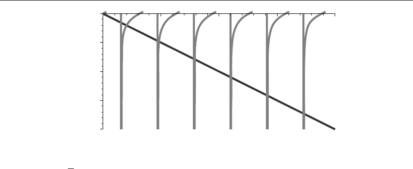
> plot({tan(z),−z},z=0..20,y=−20..0,thickness=10);
Nonhomogeneous Partial Differential Equations 505
25
210
215
220
0
y
z
5101520
Figure 8.3
If we set z =
√
λa, then the eigenvalues λ
n
are the values of z at the intersection points of the
curves shown in Figure 8.3. A few of the eigenvalues using the Maple fsolve command are
evaluated here:
> lambda[1]:=(1/aˆ2)*(fsolve((tan(z)+z),z=1..3)ˆ2);
λ
1
:= 4.115858365 (8.64)
> lambda[2]:=(1/aˆ2)*(fsolve((tan(z)+z),z=3..6)ˆ2);
λ
2
:= 24.13934203 (8.65)
> lambda[3]:=(1/aˆ2)*(fsolve((tan(z)+z),z=6..9)ˆ2);
λ
3
:= 63.65910654 (8.66)
First few terms of sum
> u(x,t):=s(x,t)+sum(v[n](x,t),n=1..3):
ANIMATION
> animate(u(x,t),x=0..a,t=0..5,thickness=3);
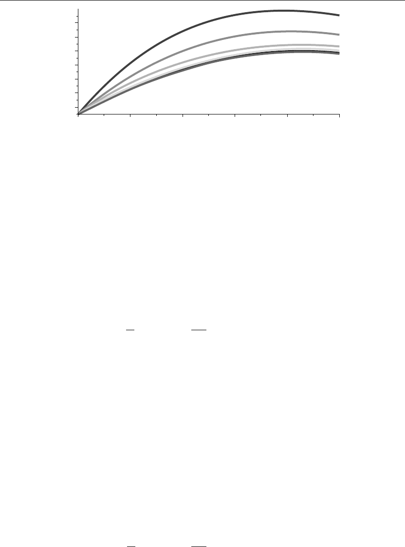
The preceding animation command displays the spatial-time-dependent solution of u(x, t) for
the given boundary conditions and initial conditions. The animation sequence here and in
Figure 8.4 shows snapshots of the animation at times t = 0, 1, 2, 3, 4, 5. Note how the solution
satisfies the given boundary and initial conditions.
ANIMATION SEQUENCE
> u(x,0):=subs(t=0,u(x,t)):u(x,1):=subs(t=1,u(x,t)):
> u(x,2):=subs(t=2,u(x,t)):u(x,3):=subs(t=3,u(x,t)):
> u(x,4):=subs(t=4,u(x,t)):u(x,5):=subs(t=5,u(x,t)):
> plot({u(x,0),u(x,1),u(x,2),u(x,3),u(x,4),u(x,5),x=0..a,thickness=10);
506 Chapter 8
18
16
14
12
10
8
6
0 0.2 0.4
x
0.6 0.8 1
Figure 8.4
EXAMPLE 8.4.4: (Electrical heating of a rod) We seek the temperature distribution in a thin
rod whose lateral surface is insulated over the interval I ={x |0 <x<1}. The left and right
ends of the rod are held at the fixed temperature of zero. The center of the rod is embedded
with a wire whose winding pitch decreases linearly with x (the space between windings
decreases linearly). The wire is electrically excited by a constant voltage source that is
switched into the circuit at time t = 0. The resistive heating effect of the wire gives rise to an
internal heat source term h(x, t) given as follows. The thermal diffusivity of the rod is
k = 1/40, and the initial temperature distribution u(x, 0) = f(x) is given here.
SOLUTION: The nonhomogeneous diffusion equation is
∂
∂t
u(x, t) = k
∂
2
∂x
2
u(x, t)
+h(x, t)
The boundary conditions are homogeneous type 1 at the left and homogeneous type 1 at the
right:
u(0,t)= 0 and u(1,t)= 0
The initial condition is
u(x, 0) = 0
The internal heat source term is
h(x, t) = xt
The solution is u(x, t) = v(x, t) +s(x, t), where s(x, t) is the linear portion of the solution
and v(x, t) is the variable portion of the solution, which satisfies the partial differential
equation
∂
∂t
v(x, t) = k
∂
2
∂x
2
v(x, t)
+q(x, t)

Nonhomogeneous Partial Differential Equations 507
where
q(x, t) = h(x, t) −
∂
∂t
s(x, t)
Assignment of system parameters
> restart: with(plots):a:=1:k:=1/40:h(x,t):=x*t:
> A(t):=0:B(t):=0:kappa[1]:=1:kappa[2]:=0:kappa[3]:=1:kappa[4]:=0:
> b(t):=(kappa[3]*a*A(t)+A(t)*kappa[4]−B(t)*kappa[2])/(kappa[1]*kappa[3]*a+
kappa[1]*kappa[4]−kappa[2]*kappa[3]);
b(t) := 0 (8.67)
> m(t):=(kappa[1]*B(t)−A(t)*kappa[3])/(kappa[1]*kappa[3]*a+kappa[1]*kappa[4]−
kappa[2]*kappa[3]);
m(t) := 0 (8.68)
Linear portion of solution
> s(x,t):=m(t)*x+b(t);s(x,0):=eval(subs(t=0,s(x,t))):
s(x, t) := 0 (8.69)
By the method of separation of variables, the variable solution is
v(x, t) =
∞
n=0
X
n
(x)T
n
(t)
where T
n
(t) is the solution to the time-dependent differential equation
d
dt
T
n
(t) +kλ
n
T
n
(t) = Q
n
(t)
and X
n
(x) is the solution to the spatial-dependent eigenvalue equation
d
2
dx
2
X
n
(x) +λ
n
X
n
(x) = 0
with boundary conditions
X(0) = 0 and X(1) = 0
The corresponding homogeneous eigenfunction problem consists of the Euler equation, along
with the homogeneous boundary conditions that are type 1 at the left and type 1 at the right.
The allowed eigenvalues and corresponding orthonormal eigenfunctions are obtained from
Example 2.5.1.