Banner A. The Calculus Lifesaver: All the Tools You Need to Excel at Calculus
Подождите немного. Документ загружается.

426 • Techniques of Integration, Part Two
Remember, this only applies when x > 0. We’ll revisit this example in Sec-
tion 19.3.6 to see how to take care of the case when x ≤ 0.
19.3.4 Completing the square and trig substitutions
Now, one other important point before we summarize the situation. From
time to time, you might want to solve an integral involving an odd power
of
√
±x
2
+ ax + b. That is, you now have a linear term ax to complicate
matters. The technique is simple: complete the square first and substitute
to get it into one of the three types that we’ve investigated. For example, to
evaluate
PSfrag
replacements
(
a, b)
[
a, b]
(
a, b]
[
a, b)
(
a, ∞)
[
a, ∞)
(
−∞, b)
(
−∞, b]
(
−∞, ∞)
{
x : a < x < b}
{
x : a ≤ x ≤ b}
{
x : a < x ≤ b}
{
x : a ≤ x < b}
{
x : x ≥ a}
{
x : x > a}
{
x : x ≤ b}
{
x : x < b}
R
a
b
shado
w
0
1
4
−
2
3
−
3
g(
x) = x
2
f(
x) = x
3
g(
x) = x
2
f(
x) = x
3
mirror
(y = x)
f
−
1
(x) =
3
√
x
y = h
(x)
y = h
−
1
(x)
y =
(x − 1)
2
−
1
x
Same
height
−
x
Same
length,
opp
osite signs
y = −
2x
−
2
1
y =
1
2
x − 1
2
−
1
y =
2
x
y =
10
x
y =
2
−x
y =
log
2
(x)
4
3
units
mirror
(x-axis)
y = |
x|
y = |
log
2
(x)|
θ radians
θ units
30
◦
=
π
6
45
◦
=
π
4
60
◦
=
π
3
120
◦
=
2
π
3
135
◦
=
3
π
4
150
◦
=
5
π
6
90
◦
=
π
2
180
◦
= π
210
◦
=
7
π
6
225
◦
=
5
π
4
240
◦
=
4
π
3
270
◦
=
3
π
2
300
◦
=
5
π
3
315
◦
=
7
π
4
330
◦
=
11
π
6
0
◦
=
0 radians
θ
hypotenuse
opp
osite
adjacen
t
0
(≡ 2π)
π
2
π
3
π
2
I
I
I
I
II
IV
θ
(
x, y)
x
y
r
7
π
6
reference
angle
reference
angle =
π
6
sin
+
sin −
cos
+
cos −
tan
+
tan −
A
S
T
C
7
π
4
9
π
13
5
π
6
(this
angle is
5π
6
clo
ckwise)
1
2
1
2
3
4
5
6
0
−
1
−
2
−
3
−
4
−
5
−
6
−
3π
−
5
π
2
−
2π
−
3
π
2
−
π
−
π
2
3
π
3
π
5
π
2
2
π
3
π
2
π
π
2
y =
sin(x)
1
0
−
1
−
3π
−
5
π
2
−
2π
−
3
π
2
−
π
−
π
2
3
π
5
π
2
2
π
2
π
3
π
2
π
π
2
y =
sin(x)
y =
cos(x)
−
π
2
π
2
y =
tan(x), −
π
2
<
x <
π
2
0
−
π
2
π
2
y =
tan(x)
−
2π
−
3π
−
5
π
2
−
3
π
2
−
π
−
π
2
π
2
3
π
3
π
5
π
2
2
π
3
π
2
π
y =
sec(x)
y =
csc(x)
y =
cot(x)
y = f(
x)
−
1
1
2
y = g(
x)
3
y = h
(x)
4
5
−
2
f(
x) =
1
x
g(
x) =
1
x
2
etc.
0
1
π
1
2
π
1
3
π
1
4
π
1
5
π
1
6
π
1
7
π
g(
x) = sin
1
x
1
0
−
1
L
10
100
200
y =
π
2
y = −
π
2
y =
tan
−1
(x)
π
2
π
y =
sin(
x)
x
,
x > 3
0
1
−
1
a
L
f(
x) = x sin (1/x)
(0 <
x < 0.3)
h
(x) = x
g(
x) = −x
a
L
lim
x
→a
+
f(x) = L
lim
x
→a
+
f(x) = ∞
lim
x
→a
+
f(x) = −∞
lim
x
→a
+
f(x) DNE
lim
x
→a
−
f(x) = L
lim
x
→a
−
f(x) = ∞
lim
x
→a
−
f(x) = −∞
lim
x
→a
−
f(x) DNE
M
}
lim
x
→a
−
f(x) = M
lim
x
→a
f(x) = L
lim
x
→a
f(x) DNE
lim
x
→∞
f(x) = L
lim
x
→∞
f(x) = ∞
lim
x
→∞
f(x) = −∞
lim
x
→∞
f(x) DNE
lim
x
→−∞
f(x) = L
lim
x
→−∞
f(x) = ∞
lim
x
→−∞
f(x) = −∞
lim
x
→−∞
f(x) DNE
lim
x →a
+
f(
x) = ∞
lim
x →a
+
f(
x) = −∞
lim
x →a
−
f(
x) = ∞
lim
x →a
−
f(
x) = −∞
lim
x →a
f(
x) = ∞
lim
x →a
f(
x) = −∞
lim
x →a
f(
x) DNE
y = f (
x)
a
y =
|
x|
x
1
−
1
y =
|
x + 2|
x +
2
1
−
1
−
2
1
2
3
4
a
a
b
y = x sin
1
x
y = x
y = −
x
a
b
c
d
C
a
b
c
d
−
1
0
1
2
3
time
y
t
u
(
t, f(t))
(
u, f(u))
time
y
t
u
y
x
(
x, f(x))
y = |
x|
(
z, f(z))
z
y = f(
x)
a
tangen
t at x = a
b
tangen
t at x = b
c
tangen
t at x = c
y = x
2
tangen
t
at x = −
1
u
v
uv
u +
∆u
v +
∆v
(
u + ∆u)(v + ∆v)
∆
u
∆
v
u
∆v
v∆
u
∆
u∆v
y = f(
x)
1
2
−
2
y = |
x
2
− 4|
y = x
2
− 4
y = −
2x + 5
y = g(
x)
1
2
3
4
5
6
7
8
9
0
−
1
−
2
−
3
−
4
−
5
−
6
y = f (
x)
3
−
3
3
−
3
0
−
1
2
easy
hard
flat
y = f
0
(
x)
3
−
3
0
−
1
2
1
−
1
y =
sin(x)
y = x
x
A
B
O
1
C
D
sin(
x)
tan(
x)
y =
sin(
x)
x
π
2
π
1
−
1
x =
0
a =
0
x
> 0
a
> 0
x
< 0
a
< 0
rest
position
+
−
y = x
2
sin
1
x
N
A
B
H
a
b
c
O
H
A
B
C
D
h
r
R
θ
1000
2000
α
β
p
h
y = g(
x) = log
b
(x)
y = f(
x) = b
x
y = e
x
5
10
1
2
3
4
0
−
1
−
2
−
3
−
4
y =
ln(x)
y =
cosh(x)
y =
sinh(x)
y =
tanh(x)
y =
sech(x)
y =
csch(x)
y =
coth(x)
1
−
1
y = f(
x)
original
function
in
verse function
slop
e = 0 at (x, y)
slop
e is infinite at (y, x)
−
108
2
5
1
2
1
2
3
4
5
6
0
−
1
−
2
−
3
−
4
−
5
−
6
−
3π
−
5
π
2
−
2π
−
3
π
2
−
π
−
π
2
3
π
3
π
5
π
2
2
π
3
π
2
π
π
2
y =
sin(x)
1
0
−
1
−
3π
−
5
π
2
−
2π
−
3
π
2
−
π
−
π
2
3
π
5
π
2
2
π
2
π
3
π
2
π
π
2
y =
sin(x)
y =
sin(x), −
π
2
≤ x ≤
π
2
−
2
−
1
0
2
π
2
−
π
2
y =
sin
−1
(x)
y =
cos(x)
π
π
2
y =
cos
−1
(x)
−
π
2
1
x
α
β
y =
tan(x)
y =
tan(x)
1
y =
tan
−1
(x)
y =
sec(x)
y =
sec
−1
(x)
y =
csc
−1
(x)
y =
cot
−1
(x)
1
y =
cosh
−1
(x)
y =
sinh
−1
(x)
y =
tanh
−1
(x)
y =
sech
−1
(x)
y =
csch
−1
(x)
y =
coth
−1
(x)
(0
, 3)
(2
, −1)
(5
, 2)
(7
, 0)
(
−1, 44)
(0
, 1)
(1
, −12)
(2
, 305)
y =
1
2
(2
, 3)
y = f(
x)
y = g(
x)
a
b
c
a
b
c
s
c
0
c
1
(
a, f(a))
(
b, f(b))
1
2
1
2
3
4
5
6
0
−
1
−
2
−
3
−
4
−
5
−
6
−
3π
−
5
π
2
−
2π
−
3
π
2
−
π
−
π
2
3
π
3
π
5
π
2
2
π
3
π
2
π
π
2
y =
sin(x)
1
0
−
1
−
3π
−
5
π
2
−
2π
−
3
π
2
−
π
−
π
2
3
π
5
π
2
2
π
2
π
3
π
2
π
π
2
c
OR
Lo
cal maximum
Lo
cal minimum
Horizon
tal point of inflection
1
e
y = f
0
(
x)
y = f (
x) = x ln(x)
−
1
e
?
y = f(
x) = x
3
y = g(
x) = x
4
x
f(
x)
−
3
−
2
−
1
0
1
2
1
2
3
4
+
−
?
1
5
6
3
f
0
(
x)
2 −
1
2
√
6
2
+
1
2
√
6
f
00
(
x)
7
8
g
00
(
x)
f
00
(
x)
0
y =
(
x − 3)(x − 1)
2
x
3
(
x + 2)
y = x ln
(x)
1
e
−
1
e
5
−
108
2
α
β
2 −
1
2
√
6
2
+
1
2
√
6
y = x
2
(
x − 5)
3
−
e
−
1/2
√
3
e
−
1/2
√
3
−
e
−3/2
e
−
3/2
−
1
√
3
1
√
3
−
1
1
y = xe
−
3x
2
/2
y =
x
3
− 6
x
2
+ 13x − 8
x
28
2
600
500
400
300
200
100
0
−
100
−
200
−
300
−
400
−
500
−
600
0
10
−
10
5
−
5
20
−
20
15
−
15
0
4
5
6
x
P
0
(
x)
+
−
−
existing
fence
new
fence
enclosure
A
h
b
H
99
100
101
h
dA/dh
r
h
1
2
7
shallo
w
deep
LAND
SEA
N
y
z
s
t
3
11
9
L
(11)
√
11
y = L
(x)
y = f (
x)
11
y = L
(x)
y = f(
x)
F
P
a
a +
∆x
f(
a + ∆x)
L
(a + ∆x)
f(
a)
error
d
f
∆
x
a
b
y = f(
x)
true
zero
starting
approximation
b
etter approximation
v
t
3
5
50
40
60
4
20
30
25
t
1
t
2
t
3
t
4
t
n
−2
t
n
−1
t
0
= a
t
n
= b
v
1
v
2
v
3
v
4
v
n
−1
v
n
−
30
6
30
|
v|
a
b
p
q
c
v(
c)
v(
c
1
)
v(
c
2
)
v(
c
3
)
v(
c
4
)
v(
c
5
)
v(
c
6
)
t
1
t
2
t
3
t
4
t
5
c
1
c
2
c
3
c
4
c
5
c
6
t
0
=
a
t
6
=
b
t
16
=
b
t
10
=
b
a
b
x
y
y = f(
x)
1
2
y = x
5
0
−
2
y =
1
a
b
y =
sin(x)
π
−
π
0
−
1
−
2
0
2
4
y = x
2
0
1
2
3
4
2
n
4
n
6
n
2(
n−2)
n
2(
n−1)
n
2
n
n
=
2
width
of each interval =
2
n
−
2
1
3
0
I
I
I
I
II
IV
4
y
dx
y = −
x
2
− 2x + 3
3
−
5
y = |−
x
2
− 2x + 3|
I
I
I
I
Ia
5
3
0
1
2
a
b
y = f (
x)
y = g(
x)
y = x
2
a
b
5
3
0
1
2
y =
√
x
2
√
2
2
2
dy
x
2
a
b
y = f(
x)
y = g(
x)
M
m
1
2
−
1
−
2
0
y = e
−
x
2
1
2
e
−1/4
f
av
y = f
av
c
A
M
0
1
2
a
b
x
t
y = f (t)
F (x )
y = f (t)
F (x + h)
x + h
F (x + h) − F (x)
f(x)
1
2
y = sin(x)
π
−π
−1
−2
y =
1
x
y = x
2
1
2
1
−1
y = ln|x|
θ
a
x
a
x
p
a
2
− x
2
3
x
p
9 − x
2
p
x
2
+ a
2
x
a
p
x
2
+ 15
x
√
15
x
p
x
2
− a
2
a
x
p
x
2
− 4
2
Z
(x
2
− 4x + 19)
−5/2
dx,
first complete the square (see Section 1.6 of Chapter 1 for a reminder of how
to do this):
x
2
− 4x + 19 = (x
2
− 4x + 4) − 4 + 19 = (x − 2)
2
+ 15.
So the integral we want is actually
Z
((x − 2)
2
+ 15)
−5/2
dx.
Now let t = x − 2, so dt = dx, and in t-land the integral becomes
Z
(t
2
+ 15)
−5/2
dt,
which we have already done earlier in Section 19.3.2! The answer was (replac-
ing the old x by t)
1
225
t
√
t
2
+ 15
−
t
3
3(t
2
+ 15)
3/2
+ C,
so replacing t now by x − 2, we see that
Z
(x
2
− 4x + 19)
−5/2
dx =
1
225
x − 2
√
x
2
− 4x + 19
−
(x − 2)
3
3(x
2
− 4x + 19)
3/2
+ C.
The moral of the story, both here and when using partial fractions, is that
a quadratic with a linear term can be made into a quadratic without one by
completing the square and substituting.
19.3.5 Summary of trig substitutions
To summarize the three main types we’ve looked at, here’s a table that shows
the appropriate substitutions and triangles for each type:
PSfrag
replacements
(
a, b)
[
a, b]
(
a, b]
[
a, b)
(
a, ∞)
[
a, ∞)
(
−∞, b)
(
−∞, b]
(
−∞, ∞)
{
x : a < x < b}
{
x : a ≤ x ≤ b}
{
x : a < x ≤ b}
{
x : a ≤ x < b}
{
x : x ≥ a}
{
x : x > a}
{
x : x ≤ b}
{
x : x < b}
R
a
b
shado
w
0
1
4
−
2
3
−
3
g(
x) = x
2
f(
x) = x
3
g(
x) = x
2
f(
x) = x
3
mirror
(y = x)
f
−
1
(x) =
3
√
x
y = h
(x)
y = h
−
1
(x)
y =
(x − 1)
2
−
1
x
Same
height
−
x
Same
length,
opp
osite signs
y = −
2x
−
2
1
y =
1
2
x − 1
2
−
1
y =
2
x
y =
10
x
y =
2
−x
y =
log
2
(x)
4
3
units
mirror
(x-axis)
y = |
x|
y = |
log
2
(x)|
θ radians
θ units
30
◦
=
π
6
45
◦
=
π
4
60
◦
=
π
3
120
◦
=
2
π
3
135
◦
=
3
π
4
150
◦
=
5
π
6
90
◦
=
π
2
180
◦
= π
210
◦
=
7
π
6
225
◦
=
5
π
4
240
◦
=
4
π
3
270
◦
=
3
π
2
300
◦
=
5
π
3
315
◦
=
7
π
4
330
◦
=
11
π
6
0
◦
=
0 radians
θ
hypotenuse
opp
osite
adjacen
t
0
(≡ 2π)
π
2
π
3
π
2
I
I
I
I
II
IV
θ
(
x, y)
x
y
r
7
π
6
reference
angle
reference
angle =
π
6
sin
+
sin −
cos
+
cos −
tan
+
tan −
A
S
T
C
7
π
4
9
π
13
5
π
6
(this
angle is
5π
6
clo
ckwise)
1
2
1
2
3
4
5
6
0
−
1
−
2
−
3
−
4
−
5
−
6
−
3π
−
5
π
2
−
2π
−
3
π
2
−
π
−
π
2
3
π
3
π
5
π
2
2
π
3
π
2
π
π
2
y =
sin(x)
1
0
−
1
−
3π
−
5
π
2
−
2π
−
3
π
2
−
π
−
π
2
3
π
5
π
2
2
π
2
π
3
π
2
π
π
2
y =
sin(x)
y =
cos(x)
−
π
2
π
2
y =
tan(x), −
π
2
<
x <
π
2
0
−
π
2
π
2
y =
tan(x)
−
2π
−
3π
−
5
π
2
−
3
π
2
−
π
−
π
2
π
2
3
π
3
π
5
π
2
2
π
3
π
2
π
y =
sec(x)
y =
csc(x)
y =
cot(x)
y = f (
x)
−
1
1
2
y = g(
x)
3
y = h
(x)
4
5
−
2
f(
x) =
1
x
g(
x) =
1
x
2
etc.
0
1
π
1
2
π
1
3
π
1
4
π
1
5
π
1
6
π
1
7
π
g(
x) = sin
1
x
1
0
−
1
L
10
100
200
y =
π
2
y = −
π
2
y =
tan
−1
(x)
π
2
π
y =
sin(
x)
x
,
x > 3
0
1
−
1
a
L
f(
x) = x sin (1/x)
(0 <
x < 0.3)
h
(x) = x
g(
x) = −x
a
L
lim
x
→a
+
f(x) = L
lim
x
→a
+
f(x) = ∞
lim
x
→a
+
f(x) = −∞
lim
x
→a
+
f(x) DNE
lim
x
→a
−
f(x) = L
lim
x
→a
−
f(x) = ∞
lim
x
→a
−
f(x) = −∞
lim
x
→a
−
f(x) DNE
M
}
lim
x
→a
−
f(x) = M
lim
x
→a
f(x) = L
lim
x
→a
f(x) DNE
lim
x
→∞
f(x) = L
lim
x
→∞
f(x) = ∞
lim
x
→∞
f(x) = −∞
lim
x
→∞
f(x) DNE
lim
x
→−∞
f(x) = L
lim
x
→−∞
f(x) = ∞
lim
x
→−∞
f(x) = −∞
lim
x
→−∞
f(x) DNE
lim
x →a
+
f(
x) = ∞
lim
x →a
+
f(
x) = −∞
lim
x →a
−
f(
x) = ∞
lim
x →a
−
f(
x) = −∞
lim
x →a
f(
x) = ∞
lim
x →a
f(
x) = −∞
lim
x →a
f(
x) DNE
y = f (
x)
a
y =
|
x|
x
1
−
1
y =
|
x + 2|
x +
2
1
−
1
−
2
1
2
3
4
a
a
b
y = x sin
1
x
y = x
y = −
x
a
b
c
d
C
a
b
c
d
−
1
0
1
2
3
time
y
t
u
(
t, f(t))
(
u, f(u))
time
y
t
u
y
x
(
x, f(x))
y = |
x|
(
z, f(z))
z
y = f (
x)
a
tangen
t at x = a
b
tangen
t at x = b
c
tangen
t at x = c
y = x
2
tangen
t
at x = −
1
u
v
uv
u +
∆u
v +
∆v
(
u + ∆u)(v + ∆v)
∆
u
∆
v
u
∆v
v∆
u
∆
u∆v
y = f (
x)
1
2
−
2
y = |
x
2
− 4|
y = x
2
− 4
y = −
2x + 5
y = g(
x)
1
2
3
4
5
6
7
8
9
0
−
1
−
2
−
3
−
4
−
5
−
6
y = f (
x)
3
−
3
3
−
3
0
−
1
2
easy
hard
flat
y = f
0
(
x)
3
−
3
0
−
1
2
1
−
1
y =
sin(x)
y = x
x
A
B
O
1
C
D
sin(
x)
tan(
x)
y =
sin
(x)
x
π
2
π
1
−
1
x =
0
a =
0
x
> 0
a
> 0
x
< 0
a
< 0
rest
position
+
−
y = x
2
sin
1
x
N
A
B
H
a
b
c
O
H
A
B
C
D
h
r
R
θ
1000
2000
α
β
p
h
y = g(
x) = log
b
(x)
y = f (
x) = b
x
y = e
x
5
10
1
2
3
4
0
−
1
−
2
−
3
−
4
y =
ln(x)
y =
cosh(x)
y =
sinh(x)
y =
tanh(x)
y =
sech(x)
y =
csch(x)
y =
coth(x)
1
−
1
y = f (
x)
original
function
in
verse function
slop
e = 0 at (x, y)
slop
e is infinite at (y, x)
−
108
2
5
1
2
1
2
3
4
5
6
0
−
1
−
2
−
3
−
4
−
5
−
6
−
3π
−
5
π
2
−
2π
−
3
π
2
−
π
−
π
2
3
π
3
π
5
π
2
2
π
3
π
2
π
π
2
y =
sin(x)
1
0
−
1
−
3π
−
5
π
2
−
2π
−
3
π
2
−
π
−
π
2
3
π
5
π
2
2
π
2
π
3
π
2
π
π
2
y =
sin(x)
y =
sin(x), −
π
2
≤ x ≤
π
2
−
2
−
1
0
2
π
2
−
π
2
y =
sin
−1
(x)
y =
cos(x)
π
π
2
y =
cos
−1
(x)
−
π
2
1
x
α
β
y =
tan(x)
y =
tan(x)
1
y =
tan
−1
(x)
y =
sec(x)
y =
sec
−1
(x)
y =
csc
−1
(x)
y =
cot
−1
(x)
1
y =
cosh
−1
(x)
y =
sinh
−1
(x)
y =
tanh
−1
(x)
y =
sech
−1
(x)
y =
csch
−1
(x)
y =
coth
−1
(x)
(0
, 3)
(2
, −1)
(5
, 2)
(7
, 0)
(
−1, 44)
(0
, 1)
(1
, −12)
(2
, 305)
y =
1
2
(2
, 3)
y = f (
x)
y = g(
x)
a
b
c
a
b
c
s
c
0
c
1
(
a, f(a))
(
b, f(b))
1
2
1
2
3
4
5
6
0
−
1
−
2
−
3
−
4
−
5
−
6
−
3π
−
5
π
2
−
2π
−
3
π
2
−
π
−
π
2
3
π
3
π
5
π
2
2
π
3
π
2
π
π
2
y =
sin(x)
1
0
−
1
−
3π
−
5
π
2
−
2π
−
3
π
2
−
π
−
π
2
3
π
5
π
2
2
π
2
π
3
π
2
π
π
2
c
OR
Lo
cal maximum
Lo
cal minimum
Horizon
tal point of inflection
1
e
y = f
0
(
x)
y = f(
x) = x ln(x)
−
1
e
?
y = f(
x) = x
3
y = g(
x) = x
4
x
f(
x)
−
3
−
2
−
1
0
1
2
1
2
3
4
+
−
?
1
5
6
3
f
0
(
x)
2 −
1
2
√
6
2
+
1
2
√
6
f
00
(
x)
7
8
g
00
(
x)
f
00
(
x)
0
y =
(
x − 3)(x − 1)
2
x
3
(
x + 2)
y = x ln
(x)
1
e
−
1
e
5
−
108
2
α
β
2 −
1
2
√
6
2
+
1
2
√
6
y = x
2
(
x − 5)
3
−
e
−
1/2
√
3
e
−
1/2
√
3
−
e
−3/2
e
−
3/2
−
1
√
3
1
√
3
−
1
1
y = xe
−
3x
2
/2
y =
x
3
− 6
x
2
+ 13x − 8
x
28
2
600
500
400
300
200
100
0
−
100
−
200
−
300
−
400
−
500
−
600
0
10
−
10
5
−
5
20
−
20
15
−
15
0
4
5
6
x
P
0
(
x)
+
−
−
existing
fence
new
fence
enclosure
A
h
b
H
99
100
101
h
dA/dh
r
h
1
2
7
shallo
w
deep
LAND
SEA
N
y
z
s
t
3
11
9
L
(11)
√
11
y = L
(x)
y = f (
x)
11
y = L
(x)
y = f (
x)
F
P
a
a +
∆x
f(
a + ∆x)
L
(a + ∆x)
f(
a)
error
d
f
∆
x
a
b
y = f (
x)
true
zero
starting
approximation
b
etter approximation
v
t
3
5
50
40
60
4
20
30
25
t
1
t
2
t
3
t
4
t
n
−2
t
n
−1
t
0
= a
t
n
= b
v
1
v
2
v
3
v
4
v
n
−1
v
n
−
30
6
30
|
v|
a
b
p
q
c
v(
c)
v(
c
1
)
v(
c
2
)
v(
c
3
)
v(
c
4
)
v(
c
5
)
v(
c
6
)
t
1
t
2
t
3
t
4
t
5
c
1
c
2
c
3
c
4
c
5
c
6
t
0
=
a
t
6
=
b
t
16
=
b
t
10
=
b
a
b
x
y
y = f (
x)
1
2
y = x
5
0
−
2
y =
1
a
b
y =
sin(x)
π
−
π
0
−
1
−
2
0
2
4
y = x
2
0
1
2
3
4
2
n
4
n
6
n
2(
n−2)
n
2(
n−1)
n
2
n
n
=
2
width
of each interval =
2
n
−
2
1
3
0
I
I
I
I
II
IV
4
y
dx
y = −
x
2
− 2x + 3
3
−
5
y = |−
x
2
− 2x + 3|
I
I
I
IIa
5
3
0
1
2
a
b
y = f (x)
y = g(x)
y = x
2
a
b
5
3
0
1
2
y =
√
x
2
√
2
2
2
dy
x
2
a
b
y = f (x)
y = g(x)
M
m
1
2
−1
−2
0
y = e
−x
2
1
2
e
−1/4
f
av
y = f
av
c
A
M
0
1
2
a
b
x
t
y = f(t)
F (x )
y = f(t)
F (x + h )
x + h
F (x + h) − F (x)
f(x)
1
2
y = sin(x)
π
−π
−1
−2
y =
1
x
y = x
2
1
2
1
−1
y = ln|x|
θ
a
x
a
x
p
a
2
− x
2
3
x
p
9 − x
2
p
x
2
+ a
2
x
a
p
x
2
+ 15
x
√
15
x
p
x
2
− a
2
a
x
p
x
2
− 4
2
Section 19.3.6: Technicalities of square roots and trig substitutions • 427
Type 1:
p
a
2
− x
2
Type 2:
p
x
2
+ a
2
Type 3:
p
x
2
− a
2
Set x = a sin(θ) Set x = a tan(θ) Set x = a sec(θ)
dx = a cos(θ) dθ dx = a sec
2
(θ) dθ dx = a sec(θ) tan(θ) dθ
a
2
− x
2
= a
2
cos
2
(θ) x
2
+ a
2
= a
2
sec
2
(θ) x
2
− a
2
= a
2
tan
2
(θ)
PSfrag
replacements
(
a, b)
[
a, b]
(
a, b]
[
a, b)
(
a, ∞)
[
a, ∞)
(
−∞, b)
(
−∞, b]
(
−∞, ∞)
{
x : a < x < b}
{
x : a ≤ x ≤ b}
{
x : a < x ≤ b}
{
x : a ≤ x < b}
{
x : x ≥ a}
{
x : x > a}
{
x : x ≤ b}
{
x : x < b}
R
a
b
shado
w
0
1
4
−
2
3
−
3
g(
x) = x
2
f(
x) = x
3
g(
x) = x
2
f(
x) = x
3
mirror
(y = x)
f
−
1
(x) =
3
√
x
y = h
(x)
y = h
−
1
(x)
y =
(x − 1)
2
−
1
x
Same
height
−
x
Same
length,
opp
osite signs
y = −
2x
−
2
1
y =
1
2
x − 1
2
−
1
y =
2
x
y =
10
x
y =
2
−x
y =
log
2
(x)
4
3
units
mirror
(x-axis)
y = |
x|
y = |
log
2
(x)|
θ radians
θ units
30
◦
=
π
6
45
◦
=
π
4
60
◦
=
π
3
120
◦
=
2
π
3
135
◦
=
3
π
4
150
◦
=
5
π
6
90
◦
=
π
2
180
◦
= π
210
◦
=
7
π
6
225
◦
=
5
π
4
240
◦
=
4
π
3
270
◦
=
3
π
2
300
◦
=
5
π
3
315
◦
=
7
π
4
330
◦
=
11
π
6
0
◦
=
0 radians
θ
hypotenuse
opp
osite
adjacen
t
0
(≡ 2π)
π
2
π
3
π
2
I
I
I
I
II
IV
θ
(
x, y)
x
y
r
7
π
6
reference
angle
reference
angle =
π
6
sin
+
sin −
cos
+
cos −
tan
+
tan −
A
S
T
C
7
π
4
9
π
13
5
π
6
(this
angle is
5π
6
clo
ckwise)
1
2
1
2
3
4
5
6
0
−
1
−
2
−
3
−
4
−
5
−
6
−
3π
−
5
π
2
−
2π
−
3
π
2
−
π
−
π
2
3
π
3
π
5
π
2
2
π
3
π
2
π
π
2
y =
sin(x)
1
0
−
1
−
3π
−
5
π
2
−
2π
−
3
π
2
−
π
−
π
2
3
π
5
π
2
2
π
2
π
3
π
2
π
π
2
y =
sin(x)
y =
cos(x)
−
π
2
π
2
y =
tan(x), −
π
2
<
x <
π
2
0
−
π
2
π
2
y =
tan(x)
−
2π
−
3π
−
5
π
2
−
3
π
2
−
π
−
π
2
π
2
3
π
3
π
5
π
2
2
π
3
π
2
π
y =
sec(x)
y =
csc(x)
y =
cot(x)
y = f(
x)
−
1
1
2
y = g(
x)
3
y = h
(x)
4
5
−
2
f(
x) =
1
x
g(
x) =
1
x
2
etc.
0
1
π
1
2
π
1
3
π
1
4
π
1
5
π
1
6
π
1
7
π
g(
x) = sin
1
x
1
0
−
1
L
10
100
200
y =
π
2
y = −
π
2
y =
tan
−1
(x)
π
2
π
y =
sin(
x)
x
,
x > 3
0
1
−
1
a
L
f(
x) = x sin (1/x)
(0 <
x < 0.3)
h
(x) = x
g(
x) = −x
a
L
lim
x
→a
+
f(x) = L
lim
x
→a
+
f(x) = ∞
lim
x
→a
+
f(x) = −∞
lim
x
→a
+
f(x) DNE
lim
x
→a
−
f(x) = L
lim
x
→a
−
f(x) = ∞
lim
x
→a
−
f(x) = −∞
lim
x
→a
−
f(x) DNE
M
}
lim
x
→a
−
f(x) = M
lim
x
→a
f(x) = L
lim
x
→a
f(x) DNE
lim
x
→∞
f(x) = L
lim
x
→∞
f(x) = ∞
lim
x
→∞
f(x) = −∞
lim
x
→∞
f(x) DNE
lim
x
→−∞
f(x) = L
lim
x
→−∞
f(x) = ∞
lim
x
→−∞
f(x) = −∞
lim
x
→−∞
f(x) DNE
lim
x →a
+
f(
x) = ∞
lim
x →a
+
f(
x) = −∞
lim
x →a
−
f(
x) = ∞
lim
x →a
−
f(
x) = −∞
lim
x →a
f(
x) = ∞
lim
x →a
f(
x) = −∞
lim
x →a
f(
x) DNE
y = f(
x)
a
y =
|
x|
x
1
−
1
y =
|
x + 2|
x +
2
1
−
1
−
2
1
2
3
4
a
a
b
y = x sin
1
x
y = x
y = −
x
a
b
c
d
C
a
b
c
d
−
1
0
1
2
3
time
y
t
u
(
t, f (t))
(
u, f (u))
time
y
t
u
y
x
(
x, f (x))
y = |
x|
(
z, f(z))
z
y = f(
x)
a
tangen
t at x = a
b
tangen
t at x = b
c
tangen
t at x = c
y = x
2
tangen
t
at x = −
1
u
v
uv
u +
∆u
v +
∆v
(
u + ∆u)(v + ∆v)
∆
u
∆
v
u
∆v
v∆
u
∆
u∆v
y = f(
x)
1
2
−
2
y = |
x
2
− 4|
y = x
2
− 4
y = −
2x + 5
y = g(
x)
1
2
3
4
5
6
7
8
9
0
−
1
−
2
−
3
−
4
−
5
−
6
y = f (
x)
3
−
3
3
−
3
0
−
1
2
easy
hard
flat
y = f
0
(
x)
3
−
3
0
−
1
2
1
−
1
y =
sin(x)
y = x
x
A
B
O
1
C
D
sin(
x)
tan(
x)
y =
sin
(x)
x
π
2
π
1
−
1
x =
0
a =
0
x
> 0
a
> 0
x
< 0
a
< 0
rest
position
+
−
y = x
2
sin
1
x
N
A
B
H
a
b
c
O
H
A
B
C
D
h
r
R
θ
1000
2000
α
β
p
h
y = g(
x) = log
b
(x)
y = f(
x) = b
x
y = e
x
5
10
1
2
3
4
0
−
1
−
2
−
3
−
4
y =
ln(x)
y =
cosh(x)
y =
sinh(x)
y =
tanh(x)
y =
sech(x)
y =
csch(x)
y =
coth(x)
1
−
1
y = f(
x)
original
function
in
verse function
slop
e = 0 at (x, y)
slop
e is infinite at (y, x)
−
108
2
5
1
2
1
2
3
4
5
6
0
−
1
−
2
−
3
−
4
−
5
−
6
−
3π
−
5
π
2
−
2π
−
3
π
2
−
π
−
π
2
3
π
3
π
5
π
2
2
π
3
π
2
π
π
2
y =
sin(x)
1
0
−
1
−
3π
−
5
π
2
−
2π
−
3
π
2
−
π
−
π
2
3
π
5
π
2
2
π
2
π
3
π
2
π
π
2
y =
sin(x)
y =
sin(x), −
π
2
≤ x ≤
π
2
−
2
−
1
0
2
π
2
−
π
2
y =
sin
−1
(x)
y =
cos(x)
π
π
2
y =
cos
−1
(x)
−
π
2
1
x
α
β
y =
tan(x)
y =
tan(x)
1
y =
tan
−1
(x)
y =
sec(x)
y =
sec
−1
(x)
y =
csc
−1
(x)
y =
cot
−1
(x)
1
y =
cosh
−1
(x)
y =
sinh
−1
(x)
y =
tanh
−1
(x)
y =
sech
−1
(x)
y =
csch
−1
(x)
y =
coth
−1
(x)
(0
, 3)
(2
, −1)
(5
, 2)
(7
, 0)
(
−1, 44)
(0
, 1)
(1
, −12)
(2
, 305)
y =
1
2
(2
, 3)
y = f(
x)
y = g(
x)
a
b
c
a
b
c
s
c
0
c
1
(
a, f (a))
(
b, f (b))
1
2
1
2
3
4
5
6
0
−
1
−
2
−
3
−
4
−
5
−
6
−
3π
−
5
π
2
−
2π
−
3
π
2
−
π
−
π
2
3
π
3
π
5
π
2
2
π
3
π
2
π
π
2
y =
sin(x)
1
0
−
1
−
3π
−
5
π
2
−
2π
−
3
π
2
−
π
−
π
2
3
π
5
π
2
2
π
2
π
3
π
2
π
π
2
c
OR
Lo
cal maximum
Lo
cal minimum
Horizon
tal point of inflection
1
e
y = f
0
(
x)
y = f (
x) = x ln(x)
−
1
e
?
y = f(
x) = x
3
y = g(
x) = x
4
x
f(
x)
−
3
−
2
−
1
0
1
2
1
2
3
4
+
−
?
1
5
6
3
f
0
(
x)
2 −
1
2
√
6
2
+
1
2
√
6
f
00
(
x)
7
8
g
00
(
x)
f
00
(
x)
0
y =
(
x − 3)(x − 1)
2
x
3
(
x + 2)
y = x ln
(x)
1
e
−
1
e
5
−
108
2
α
β
2 −
1
2
√
6
2
+
1
2
√
6
y = x
2
(
x − 5)
3
−
e
−
1/2
√
3
e
−
1/2
√
3
−
e
−3/2
e
−
3/2
−
1
√
3
1
√
3
−
1
1
y = xe
−
3x
2
/2
y =
x
3
− 6
x
2
+ 13x − 8
x
28
2
600
500
400
300
200
100
0
−
100
−
200
−
300
−
400
−
500
−
600
0
10
−
10
5
−
5
20
−
20
15
−
15
0
4
5
6
x
P
0
(
x)
+
−
−
existing
fence
new
fence
enclosure
A
h
b
H
99
100
101
h
dA/dh
r
h
1
2
7
shallo
w
deep
LAND
SEA
N
y
z
s
t
3
11
9
L
(11)
√
11
y = L
(x)
y = f (
x)
11
y = L
(x)
y = f(
x)
F
P
a
a +
∆x
f(
a + ∆x)
L
(a + ∆x)
f(
a)
error
d
f
∆
x
a
b
y = f(
x)
true
zero
starting
approximation
b
etter approximation
v
t
3
5
50
40
60
4
20
30
25
t
1
t
2
t
3
t
4
t
n
−2
t
n
−1
t
0
= a
t
n
= b
v
1
v
2
v
3
v
4
v
n
−1
v
n
−
30
6
30
|
v|
a
b
p
q
c
v(
c)
v(
c
1
)
v(
c
2
)
v(
c
3
)
v(
c
4
)
v(
c
5
)
v(
c
6
)
t
1
t
2
t
3
t
4
t
5
c
1
c
2
c
3
c
4
c
5
c
6
t
0
=
a
t
6
=
b
t
16
=
b
t
10
=
b
a
b
x
y
y = f(
x)
1
2
y = x
5
0
−
2
y =
1
a
b
y =
sin(x)
π
−
π
0
−1
−2
0
2
4
y = x
2
0
1
2
3
4
2
n
4
n
6
n
2(n−2)
n
2(n−1)
n
2n
n
= 2
width of each interval =
2
n
−2
1
3
0
I
II
III
IV
4
y
dx
y = −x
2
− 2x + 3
3
−5
y = |−x
2
− 2x + 3|
I
II
IIa
5
3
0
1
2
a
b
y = f (x)
y = g(x)
y = x
2
a
b
5
3
0
1
2
y =
√
x
2
√
2
2
2
dy
x
2
a
b
y = f(x)
y = g(x)
M
m
1
2
−1
−2
0
y = e
−x
2
1
2
e
−1/4
f
av
y = f
av
c
A
M
0
1
2
a
b
x
t
y = f(t)
F (x )
y = f(t)
F (x + h)
x + h
F (x + h) − F (x)
f(x)
1
2
y = sin(x)
π
−π
−1
−2
y =
1
x
y = x
2
1
2
1
−1
y = ln|x|
θ
a
x
a
x
p
a
2
− x
2
3
x
p
9 − x
2
p
x
2
+ a
2
x
a
p
x
2
+ 15
x
√
15
x
p
x
2
− a
2
a
x
p
x
2
− 4
2
a
x
p
a
2
− x
2
PSfrag
replacements
(
a, b)
[
a, b]
(
a, b]
[
a, b)
(
a, ∞)
[
a, ∞)
(
−∞, b)
(
−∞, b]
(
−∞, ∞)
{
x : a < x < b}
{
x : a ≤ x ≤ b}
{
x : a < x ≤ b}
{
x : a ≤ x < b}
{
x : x ≥ a}
{
x : x > a}
{
x : x ≤ b}
{
x : x < b}
R
a
b
shado
w
0
1
4
−
2
3
−
3
g(
x) = x
2
f(
x) = x
3
g(
x) = x
2
f(
x) = x
3
mirror
(y = x)
f
−
1
(x) =
3
√
x
y = h
(x)
y = h
−
1
(x)
y =
(x − 1)
2
−
1
x
Same
height
−
x
Same
length,
opp
osite signs
y = −
2x
−
2
1
y =
1
2
x − 1
2
−
1
y =
2
x
y =
10
x
y =
2
−x
y =
log
2
(x)
4
3
units
mirror
(x-axis)
y = |
x|
y = |
log
2
(x)|
θ radians
θ units
30
◦
=
π
6
45
◦
=
π
4
60
◦
=
π
3
120
◦
=
2
π
3
135
◦
=
3
π
4
150
◦
=
5
π
6
90
◦
=
π
2
180
◦
= π
210
◦
=
7
π
6
225
◦
=
5
π
4
240
◦
=
4
π
3
270
◦
=
3
π
2
300
◦
=
5
π
3
315
◦
=
7
π
4
330
◦
=
11
π
6
0
◦
=
0 radians
θ
hypotenuse
opp
osite
adjacen
t
0
(≡ 2π)
π
2
π
3
π
2
I
I
I
I
II
IV
θ
(
x, y)
x
y
r
7
π
6
reference
angle
reference
angle =
π
6
sin
+
sin −
cos
+
cos −
tan
+
tan −
A
S
T
C
7
π
4
9
π
13
5
π
6
(this
angle is
5π
6
clo
ckwise)
1
2
1
2
3
4
5
6
0
−
1
−
2
−
3
−
4
−
5
−
6
−
3π
−
5
π
2
−
2π
−
3
π
2
−
π
−
π
2
3
π
3
π
5
π
2
2
π
3
π
2
π
π
2
y =
sin(x)
1
0
−
1
−
3π
−
5
π
2
−
2π
−
3
π
2
−
π
−
π
2
3
π
5
π
2
2
π
2
π
3
π
2
π
π
2
y =
sin(x)
y =
cos(x)
−
π
2
π
2
y =
tan(x), −
π
2
<
x <
π
2
0
−
π
2
π
2
y =
tan(x)
−
2π
−
3π
−
5
π
2
−
3
π
2
−
π
−
π
2
π
2
3
π
3
π
5
π
2
2
π
3
π
2
π
y =
sec(x)
y =
csc(x)
y =
cot(x)
y = f(
x)
−
1
1
2
y = g(
x)
3
y = h
(x)
4
5
−
2
f(
x) =
1
x
g(
x) =
1
x
2
etc.
0
1
π
1
2
π
1
3
π
1
4
π
1
5
π
1
6
π
1
7
π
g(
x) = sin
1
x
1
0
−
1
L
10
100
200
y =
π
2
y = −
π
2
y =
tan
−1
(x)
π
2
π
y =
sin(
x)
x
,
x > 3
0
1
−
1
a
L
f(
x) = x sin (1/x)
(0 <
x < 0.3)
h
(x) = x
g(
x) = −x
a
L
lim
x
→a
+
f(x) = L
lim
x
→a
+
f(x) = ∞
lim
x
→a
+
f(x) = −∞
lim
x
→a
+
f(x) DNE
lim
x
→a
−
f(x) = L
lim
x
→a
−
f(x) = ∞
lim
x
→a
−
f(x) = −∞
lim
x
→a
−
f(x) DNE
M
}
lim
x
→a
−
f(x) = M
lim
x
→a
f(x) = L
lim
x
→a
f(x) DNE
lim
x
→∞
f(x) = L
lim
x
→∞
f(x) = ∞
lim
x
→∞
f(x) = −∞
lim
x
→∞
f(x) DNE
lim
x
→−∞
f(x) = L
lim
x
→−∞
f(x) = ∞
lim
x
→−∞
f(x) = −∞
lim
x
→−∞
f(x) DNE
lim
x →a
+
f(
x) = ∞
lim
x →a
+
f(
x) = −∞
lim
x →a
−
f(
x) = ∞
lim
x →a
−
f(
x) = −∞
lim
x →a
f(
x) = ∞
lim
x →a
f(
x) = −∞
lim
x →a
f(
x) DNE
y = f (
x)
a
y =
|
x|
x
1
−
1
y =
|
x + 2|
x +
2
1
−
1
−
2
1
2
3
4
a
a
b
y = x sin
1
x
y = x
y = −
x
a
b
c
d
C
a
b
c
d
−
1
0
1
2
3
time
y
t
u
(
t, f (t))
(
u, f (u))
time
y
t
u
y
x
(
x, f (x))
y = |
x|
(
z, f(z))
z
y = f(
x)
a
tangen
t at x = a
b
tangen
t at x = b
c
tangen
t at x = c
y = x
2
tangen
t
at x = −
1
u
v
uv
u +
∆u
v +
∆v
(
u + ∆u)(v + ∆v)
∆
u
∆
v
u
∆v
v∆
u
∆
u∆v
y = f(
x)
1
2
−
2
y = |
x
2
− 4|
y = x
2
− 4
y = −
2x + 5
y = g(
x)
1
2
3
4
5
6
7
8
9
0
−
1
−
2
−
3
−
4
−
5
−
6
y = f (
x)
3
−
3
3
−
3
0
−
1
2
easy
hard
flat
y = f
0
(
x)
3
−
3
0
−
1
2
1
−
1
y =
sin(x)
y = x
x
A
B
O
1
C
D
sin(
x)
tan(
x)
y =
sin
(x)
x
π
2
π
1
−
1
x =
0
a =
0
x
> 0
a
> 0
x
< 0
a
< 0
rest
position
+
−
y = x
2
sin
1
x
N
A
B
H
a
b
c
O
H
A
B
C
D
h
r
R
θ
1000
2000
α
β
p
h
y = g(
x) = log
b
(x)
y = f(
x) = b
x
y = e
x
5
10
1
2
3
4
0
−
1
−
2
−
3
−
4
y =
ln(x)
y =
cosh(x)
y =
sinh(x)
y =
tanh(x)
y =
sech(x)
y =
csch(x)
y =
coth(x)
1
−
1
y = f(
x)
original
function
in
verse function
slop
e = 0 at (x, y)
slop
e is infinite at (y, x)
−
108
2
5
1
2
1
2
3
4
5
6
0
−
1
−
2
−
3
−
4
−
5
−
6
−
3π
−
5
π
2
−
2π
−
3
π
2
−
π
−
π
2
3
π
3
π
5
π
2
2
π
3
π
2
π
π
2
y =
sin(x)
1
0
−
1
−
3π
−
5
π
2
−
2π
−
3
π
2
−
π
−
π
2
3
π
5
π
2
2
π
2
π
3
π
2
π
π
2
y =
sin(x)
y =
sin(x), −
π
2
≤ x ≤
π
2
−
2
−
1
0
2
π
2
−
π
2
y =
sin
−1
(x)
y =
cos(x)
π
π
2
y =
cos
−1
(x)
−
π
2
1
x
α
β
y =
tan(x)
y =
tan(x)
1
y =
tan
−1
(x)
y =
sec(x)
y =
sec
−1
(x)
y =
csc
−1
(x)
y =
cot
−1
(x)
1
y =
cosh
−1
(x)
y =
sinh
−1
(x)
y =
tanh
−1
(x)
y =
sech
−1
(x)
y =
csch
−1
(x)
y =
coth
−1
(x)
(0
, 3)
(2
, −1)
(5
, 2)
(7
, 0)
(
−1, 44)
(0
, 1)
(1
, −12)
(2
, 305)
y =
1
2
(2
, 3)
y = f(
x)
y = g(
x)
a
b
c
a
b
c
s
c
0
c
1
(
a, f (a))
(
b, f (b))
1
2
1
2
3
4
5
6
0
−
1
−
2
−
3
−
4
−
5
−
6
−
3π
−
5
π
2
−
2π
−
3
π
2
−
π
−
π
2
3
π
3
π
5
π
2
2
π
3
π
2
π
π
2
y =
sin(x)
1
0
−
1
−
3π
−
5
π
2
−
2π
−
3
π
2
−
π
−
π
2
3
π
5
π
2
2
π
2
π
3
π
2
π
π
2
c
OR
Lo
cal maximum
Lo
cal minimum
Horizon
tal point of inflection
1
e
y = f
0
(
x)
y = f (
x) = x ln(x)
−
1
e
?
y = f(
x) = x
3
y = g(
x) = x
4
x
f(
x)
−
3
−
2
−
1
0
1
2
1
2
3
4
+
−
?
1
5
6
3
f
0
(
x)
2 −
1
2
√
6
2
+
1
2
√
6
f
00
(
x)
7
8
g
00
(
x)
f
00
(
x)
0
y =
(
x − 3)(x − 1)
2
x
3
(
x + 2)
y = x ln(
x)
1
e
−
1
e
5
−
108
2
α
β
2 −
1
2
√
6
2
+
1
2
√
6
y = x
2
(
x − 5)
3
−
e
−
1/2
√
3
e
−
1/2
√
3
−
e
−3/2
e
−
3/2
−
1
√
3
1
√
3
−
1
1
y = xe
−
3x
2
/2
y =
x
3
− 6
x
2
+ 13x − 8
x
28
2
600
500
400
300
200
100
0
−
100
−
200
−
300
−
400
−
500
−
600
0
10
−
10
5
−
5
20
−
20
15
−
15
0
4
5
6
x
P
0
(
x)
+
−
−
existing
fence
new
fence
enclosure
A
h
b
H
99
100
101
h
dA/dh
r
h
1
2
7
shallo
w
deep
LAND
SEA
N
y
z
s
t
3
11
9
L
(11)
√
11
y = L
(x)
y = f (
x)
11
y = L
(x)
y = f(
x)
F
P
a
a +
∆x
f(
a + ∆x)
L
(a + ∆x)
f(
a)
error
d
f
∆
x
a
b
y = f(
x)
true
zero
starting
approximation
b
etter approximation
v
t
3
5
50
40
60
4
20
30
25
t
1
t
2
t
3
t
4
t
n
−2
t
n
−1
t
0
= a
t
n
= b
v
1
v
2
v
3
v
4
v
n
−1
v
n
−
30
6
30
|
v|
a
b
p
q
c
v(
c)
v(
c
1
)
v(
c
2
)
v(
c
3
)
v(
c
4
)
v(
c
5
)
v(
c
6
)
t
1
t
2
t
3
t
4
t
5
c
1
c
2
c
3
c
4
c
5
c
6
t
0
=
a
t
6
=
b
t
16
=
b
t
10
=
b
a
b
x
y
y = f(
x)
1
2
y = x
5
0
−
2
y =
1
a
b
y =
sin(x)
π
−
π
0
−
1
−
2
0
2
4
y = x
2
0
1
2
3
4
2
n
4
n
6
n
2(n−2)
n
2(n−1)
n
2n
n
= 2
width of each interval =
2
n
−2
1
3
0
I
II
III
IV
4
y
dx
y = −x
2
− 2x + 3
3
−5
y = |−x
2
− 2x + 3|
I
II
IIa
5
3
0
1
2
a
b
y = f (x)
y = g(x)
y = x
2
a
b
5
3
0
1
2
y =
√
x
2
√
2
2
2
dy
x
2
a
b
y = f(x)
y = g(x)
M
m
1
2
−1
−2
0
y = e
−x
2
1
2
e
−1/4
f
av
y = f
av
c
A
M
0
1
2
a
b
x
t
y = f(t)
F (x )
y = f(t)
F (x + h)
x + h
F (x + h) − F (x)
f(x)
1
2
y = sin(x)
π
−π
−1
−2
y =
1
x
y = x
2
1
2
1
−1
y = ln|x|
θ
a
x
a
x
p
a
2
− x
2
3
x
p
9 − x
2
p
x
2
+ a
2
x
a
p
x
2
+ 15
x
√
15
x
p
x
2
− a
2
a
x
p
x
2
− 4
2
p
x
2
+ a
2
x
a
PSfrag
replacements
(
a, b)
[
a, b]
(
a, b]
[
a, b)
(
a, ∞)
[
a, ∞)
(
−∞, b)
(
−∞, b]
(
−∞, ∞)
{
x : a < x < b}
{
x : a ≤ x ≤ b}
{
x : a < x ≤ b}
{
x : a ≤ x < b}
{
x : x ≥ a}
{
x : x > a}
{
x : x ≤ b}
{
x : x < b}
R
a
b
shado
w
0
1
4
−
2
3
−
3
g(
x) = x
2
f(
x) = x
3
g(
x) = x
2
f(
x) = x
3
mirror
(y = x)
f
−
1
(x) =
3
√
x
y = h
(x)
y = h
−
1
(x)
y =
(x − 1)
2
−
1
x
Same
height
−
x
Same
length,
opp
osite signs
y = −
2x
−
2
1
y =
1
2
x − 1
2
−
1
y =
2
x
y =
10
x
y =
2
−x
y =
log
2
(x)
4
3
units
mirror
(x-axis)
y = |
x|
y = |
log
2
(x)|
θ radians
θ units
30
◦
=
π
6
45
◦
=
π
4
60
◦
=
π
3
120
◦
=
2
π
3
135
◦
=
3
π
4
150
◦
=
5
π
6
90
◦
=
π
2
180
◦
= π
210
◦
=
7
π
6
225
◦
=
5
π
4
240
◦
=
4
π
3
270
◦
=
3
π
2
300
◦
=
5
π
3
315
◦
=
7
π
4
330
◦
=
11
π
6
0
◦
=
0 radians
θ
hypotenuse
opp
osite
adjacen
t
0
(≡ 2π)
π
2
π
3
π
2
I
I
I
I
II
IV
θ
(
x, y)
x
y
r
7
π
6
reference
angle
reference
angle =
π
6
sin
+
sin −
cos
+
cos −
tan
+
tan −
A
S
T
C
7
π
4
9
π
13
5
π
6
(this
angle is
5π
6
clo
ckwise)
1
2
1
2
3
4
5
6
0
−
1
−
2
−
3
−
4
−
5
−
6
−
3π
−
5
π
2
−
2π
−
3
π
2
−
π
−
π
2
3
π
3
π
5
π
2
2
π
3
π
2
π
π
2
y =
sin(x)
1
0
−
1
−
3π
−
5
π
2
−
2π
−
3
π
2
−
π
−
π
2
3
π
5
π
2
2
π
2
π
3
π
2
π
π
2
y =
sin(x)
y =
cos(x)
−
π
2
π
2
y =
tan(x), −
π
2
<
x <
π
2
0
−
π
2
π
2
y =
tan(x)
−
2π
−
3π
−
5
π
2
−
3
π
2
−
π
−
π
2
π
2
3
π
3
π
5
π
2
2
π
3
π
2
π
y =
sec(x)
y =
csc(x)
y =
cot(x)
y = f(
x)
−
1
1
2
y = g(
x)
3
y = h
(x)
4
5
−
2
f(
x) =
1
x
g(
x) =
1
x
2
etc.
0
1
π
1
2
π
1
3
π
1
4
π
1
5
π
1
6
π
1
7
π
g(
x) = sin
1
x
1
0
−
1
L
10
100
200
y =
π
2
y = −
π
2
y =
tan
−1
(x)
π
2
π
y =
sin(
x)
x
,
x > 3
0
1
−
1
a
L
f(
x) = x sin (1/x)
(0 <
x < 0.3)
h
(x) = x
g(
x) = −x
a
L
lim
x
→a
+
f(x) = L
lim
x
→a
+
f(x) = ∞
lim
x
→a
+
f(x) = −∞
lim
x
→a
+
f(x) DNE
lim
x
→a
−
f(x) = L
lim
x
→a
−
f(x) = ∞
lim
x
→a
−
f(x) = −∞
lim
x
→a
−
f(x) DNE
M
}
lim
x
→a
−
f(x) = M
lim
x
→a
f(x) = L
lim
x
→a
f(x) DNE
lim
x
→∞
f(x) = L
lim
x
→∞
f(x) = ∞
lim
x
→∞
f(x) = −∞
lim
x
→∞
f(x) DNE
lim
x
→−∞
f(x) = L
lim
x
→−∞
f(x) = ∞
lim
x
→−∞
f(x) = −∞
lim
x
→−∞
f(x) DNE
lim
x →a
+
f(
x) = ∞
lim
x →a
+
f(
x) = −∞
lim
x →a
−
f(
x) = ∞
lim
x →a
−
f(
x) = −∞
lim
x →a
f(
x) = ∞
lim
x →a
f(
x) = −∞
lim
x →a
f(
x) DNE
y = f(
x)
a
y =
|
x|
x
1
−
1
y =
|
x + 2|
x +
2
1
−
1
−
2
1
2
3
4
a
a
b
y = x sin
1
x
y = x
y = −
x
a
b
c
d
C
a
b
c
d
−
1
0
1
2
3
time
y
t
u
(
t, f (t))
(
u, f (u))
time
y
t
u
y
x
(
x, f (x))
y = |
x|
(
z, f(z))
z
y = f(
x)
a
tangen
t at x = a
b
tangen
t at x = b
c
tangen
t at x = c
y = x
2
tangen
t
at x = −
1
u
v
uv
u +
∆u
v +
∆v
(
u + ∆u)(v + ∆v)
∆
u
∆
v
u
∆v
v∆
u
∆
u∆v
y = f(
x)
1
2
−
2
y = |
x
2
− 4|
y = x
2
− 4
y = −
2x + 5
y = g(
x)
1
2
3
4
5
6
7
8
9
0
−
1
−
2
−
3
−
4
−
5
−
6
y = f(
x)
3
−
3
3
−
3
0
−
1
2
easy
hard
flat
y = f
0
(
x)
3
−
3
0
−
1
2
1
−
1
y =
sin(x)
y = x
x
A
B
O
1
C
D
sin(
x)
tan(
x)
y =
sin(
x)
x
π
2
π
1
−
1
x =
0
a =
0
x
> 0
a
> 0
x
< 0
a
< 0
rest
position
+
−
y = x
2
sin
1
x
N
A
B
H
a
b
c
O
H
A
B
C
D
h
r
R
θ
1000
2000
α
β
p
h
y = g(
x) = log
b
(x)
y = f(
x) = b
x
y = e
x
5
10
1
2
3
4
0
−
1
−
2
−
3
−
4
y =
ln(x)
y =
cosh(x)
y =
sinh(x)
y =
tanh(x)
y =
sech(x)
y =
csch(x)
y =
coth(x)
1
−
1
y = f(
x)
original
function
in
verse function
slop
e = 0 at (x, y)
slop
e is infinite at (y, x)
−
108
2
5
1
2
1
2
3
4
5
6
0
−
1
−
2
−
3
−
4
−
5
−
6
−
3π
−
5
π
2
−
2π
−
3
π
2
−
π
−
π
2
3
π
3
π
5
π
2
2
π
3
π
2
π
π
2
y =
sin(x)
1
0
−
1
−
3π
−
5
π
2
−
2π
−
3
π
2
−
π
−
π
2
3
π
5
π
2
2
π
2
π
3
π
2
π
π
2
y =
sin(x)
y =
sin(x), −
π
2
≤ x ≤
π
2
−
2
−
1
0
2
π
2
−
π
2
y =
sin
−1
(x)
y =
cos(x)
π
π
2
y =
cos
−1
(x)
−
π
2
1
x
α
β
y =
tan(x)
y =
tan(x)
1
y =
tan
−1
(x)
y =
sec(x)
y =
sec
−1
(x)
y =
csc
−1
(x)
y =
cot
−1
(x)
1
y =
cosh
−1
(x)
y =
sinh
−1
(x)
y =
tanh
−1
(x)
y =
sech
−1
(x)
y =
csch
−1
(x)
y =
coth
−1
(x)
(0
, 3)
(2
, −1)
(5
, 2)
(7
, 0)
(
−1, 44)
(0
, 1)
(1
, −12)
(2
, 305)
y =
1
2
(2
, 3)
y = f(
x)
y = g(
x)
a
b
c
a
b
c
s
c
0
c
1
(
a, f (a))
(
b, f (b))
1
2
1
2
3
4
5
6
0
−
1
−
2
−
3
−
4
−
5
−
6
−
3π
−
5
π
2
−
2π
−
3
π
2
−
π
−
π
2
3
π
3
π
5
π
2
2
π
3
π
2
π
π
2
y =
sin(x)
1
0
−
1
−
3π
−
5
π
2
−
2π
−
3
π
2
−
π
−
π
2
3
π
5
π
2
2
π
2
π
3
π
2
π
π
2
c
OR
Lo
cal maximum
Lo
cal minimum
Horizon
tal point of inflection
1
e
y = f
0
(
x)
y = f(
x) = x ln(x)
−
1
e
?
y = f(
x) = x
3
y = g(
x) = x
4
x
f(
x)
−
3
−
2
−
1
0
1
2
1
2
3
4
+
−
?
1
5
6
3
f
0
(
x)
2 −
1
2
√
6
2
+
1
2
√
6
f
00
(
x)
7
8
g
00
(
x)
f
00
(
x)
0
y =
(
x − 3)(x − 1)
2
x
3
(
x + 2)
y = x ln
(x)
1
e
−
1
e
5
−
108
2
α
β
2 −
1
2
√
6
2
+
1
2
√
6
y = x
2
(
x − 5)
3
−
e
−
1/2
√
3
e
−
1/2
√
3
−
e
−3/2
e
−
3/2
−
1
√
3
1
√
3
−
1
1
y = xe
−
3x
2
/2
y =
x
3
− 6
x
2
+ 13x − 8
x
28
2
600
500
400
300
200
100
0
−
100
−
200
−
300
−
400
−
500
−
600
0
10
−
10
5
−
5
20
−
20
15
−
15
0
4
5
6
x
P
0
(
x)
+
−
−
existing
fence
new
fence
enclosure
A
h
b
H
99
100
101
h
dA/dh
r
h
1
2
7
shallo
w
deep
LAND
SEA
N
y
z
s
t
3
11
9
L
(11)
√
11
y = L
(x)
y = f(
x)
11
y = L
(x)
y = f(
x)
F
P
a
a +
∆x
f(
a + ∆x)
L
(a + ∆x)
f(
a)
error
d
f
∆
x
a
b
y = f(
x)
true
zero
starting
approximation
b
etter approximation
v
t
3
5
50
40
60
4
20
30
25
t
1
t
2
t
3
t
4
t
n
−2
t
n
−1
t
0
= a
t
n
= b
v
1
v
2
v
3
v
4
v
n
−1
v
n
−
30
6
30
|
v|
a
b
p
q
c
v(
c)
v(
c
1
)
v(
c
2
)
v(
c
3
)
v(
c
4
)
v(
c
5
)
v(
c
6
)
t
1
t
2
t
3
t
4
t
5
c
1
c
2
c
3
c
4
c
5
c
6
t
0
=
a
t
6
=
b
t
16
=
b
t
10
=
b
a
b
x
y
y = f(
x)
1
2
y = x
5
0
−
2
y =
1
a
b
y =
sin(x)
π
−
π
0
−1
−2
0
2
4
y = x
2
0
1
2
3
4
2
n
4
n
6
n
2(n−2)
n
2(n−1)
n
2n
n
= 2
width of each interval =
2
n
−2
1
3
0
I
II
III
IV
4
y
dx
y = −x
2
− 2x + 3
3
−5
y = |−x
2
− 2x + 3|
I
II
IIa
5
3
0
1
2
a
b
y = f (x)
y = g(x)
y = x
2
a
b
5
3
0
1
2
y =
√
x
2
√
2
2
2
dy
x
2
a
b
y = f(x)
y = g(x)
M
m
1
2
−1
−2
0
y = e
−x
2
1
2
e
−1/4
f
av
y = f
av
c
A
M
0
1
2
a
b
x
t
y = f(t)
F (x )
y = f(t)
F (x + h)
x + h
F (x + h) − F (x)
f(x)
1
2
y = sin(x)
π
−π
−1
−2
y =
1
x
y = x
2
1
2
1
−1
y = ln|x|
θ
a
x
a
x
p
a
2
− x
2
3
x
p
9 − x
2
p
x
2
+ a
2
x
a
p
x
2
+ 15
x
√
15
x
p
x
2
− a
2
a
x
p
x
2
− 4
2
x
p
x
2
− a
2
a
The next section discusses the technical point about when (and why) you can
drop the absolute value signs when you take square roots of quantities like
a
2
cos
2
(θ) or a
2
tan
2
(θ). It’s the sort of thing that you may want to skim over
first, then come back to later if you have time.
19.3.6 Technicalities of square roots and trig substitutions
You have been warned: this section gets a little messy. Still with me? Good.
PSfrag
replacements
(
a, b)
[
a, b]
(
a, b]
[
a, b)
(
a, ∞)
[
a, ∞)
(
−∞, b)
(
−∞, b]
(
−∞, ∞)
{
x : a < x < b}
{
x : a ≤ x ≤ b}
{
x : a < x ≤ b}
{
x : a ≤ x < b}
{
x : x ≥ a}
{
x : x > a}
{
x : x ≤ b}
{
x : x < b}
R
a
b
shado
w
0
1
4
−
2
3
−
3
g(
x) = x
2
f(
x) = x
3
g(
x) = x
2
f(
x) = x
3
mirror
(y = x)
f
−
1
(x) =
3
√
x
y = h
(x)
y = h
−
1
(x)
y =
(x − 1)
2
−
1
x
Same
height
−
x
Same
length,
opp
osite signs
y = −
2x
−
2
1
y =
1
2
x − 1
2
−
1
y =
2
x
y =
10
x
y =
2
−x
y =
log
2
(x)
4
3
units
mirror
(x-axis)
y = |
x|
y = |
log
2
(x)|
θ radians
θ units
30
◦
=
π
6
45
◦
=
π
4
60
◦
=
π
3
120
◦
=
2
π
3
135
◦
=
3
π
4
150
◦
=
5
π
6
90
◦
=
π
2
180
◦
= π
210
◦
=
7
π
6
225
◦
=
5
π
4
240
◦
=
4
π
3
270
◦
=
3
π
2
300
◦
=
5
π
3
315
◦
=
7
π
4
330
◦
=
11
π
6
0
◦
=
0 radians
θ
hypotenuse
opp
osite
adjacen
t
0
(≡ 2π)
π
2
π
3
π
2
I
I
I
I
II
IV
θ
(
x, y)
x
y
r
7
π
6
reference
angle
reference
angle =
π
6
sin
+
sin −
cos
+
cos −
tan
+
tan −
A
S
T
C
7
π
4
9
π
13
5
π
6
(this
angle is
5π
6
clo
ckwise)
1
2
1
2
3
4
5
6
0
−
1
−
2
−
3
−
4
−
5
−
6
−
3π
−
5
π
2
−
2π
−
3
π
2
−
π
−
π
2
3
π
3
π
5
π
2
2
π
3
π
2
π
π
2
y =
sin(x)
1
0
−
1
−
3π
−
5
π
2
−
2π
−
3
π
2
−
π
−
π
2
3
π
5
π
2
2
π
2
π
3
π
2
π
π
2
y =
sin(x)
y =
cos(x)
−
π
2
π
2
y =
tan(x), −
π
2
<
x <
π
2
0
−
π
2
π
2
y =
tan(x)
−
2π
−
3π
−
5
π
2
−
3
π
2
−
π
−
π
2
π
2
3
π
3
π
5
π
2
2
π
3
π
2
π
y =
sec(x)
y =
csc(x)
y =
cot(x)
y = f(
x)
−
1
1
2
y = g(
x)
3
y = h
(x)
4
5
−
2
f(
x) =
1
x
g(
x) =
1
x
2
etc.
0
1
π
1
2
π
1
3
π
1
4
π
1
5
π
1
6
π
1
7
π
g(
x) = sin
1
x
1
0
−
1
L
10
100
200
y =
π
2
y = −
π
2
y =
tan
−1
(x)
π
2
π
y =
sin(
x)
x
,
x > 3
0
1
−
1
a
L
f(
x) = x sin (1/x)
(0 <
x < 0.3)
h
(x) = x
g(
x) = −x
a
L
lim
x
→a
+
f(x) = L
lim
x
→a
+
f(x) = ∞
lim
x
→a
+
f(x) = −∞
lim
x
→a
+
f(x) DNE
lim
x
→a
−
f(x) = L
lim
x
→a
−
f(x) = ∞
lim
x
→a
−
f(x) = −∞
lim
x
→a
−
f(x) DNE
M
}
lim
x
→a
−
f(x) = M
lim
x
→a
f(x) = L
lim
x
→a
f(x) DNE
lim
x
→∞
f(x) = L
lim
x
→∞
f(x) = ∞
lim
x
→∞
f(x) = −∞
lim
x
→∞
f(x) DNE
lim
x
→−∞
f(x) = L
lim
x
→−∞
f(x) = ∞
lim
x
→−∞
f(x) = −∞
lim
x
→−∞
f(x) DNE
lim
x →a
+
f(
x) = ∞
lim
x →a
+
f(
x) = −∞
lim
x →a
−
f(
x) = ∞
lim
x →a
−
f(
x) = −∞
lim
x →a
f(
x) = ∞
lim
x →a
f(
x) = −∞
lim
x →a
f(
x) DNE
y = f (
x)
a
y =
|
x|
x
1
−
1
y =
|
x + 2|
x +
2
1
−
1
−
2
1
2
3
4
a
a
b
y = x sin
1
x
y = x
y = −
x
a
b
c
d
C
a
b
c
d
−
1
0
1
2
3
time
y
t
u
(
t, f(t))
(
u, f(u))
time
y
t
u
y
x
(
x, f(x))
y = |
x|
(
z, f(z))
z
y = f(
x)
a
tangen
t at x = a
b
tangen
t at x = b
c
tangen
t at x = c
y = x
2
tangen
t
at x = −
1
u
v
uv
u +
∆u
v +
∆v
(
u + ∆u)(v + ∆v)
∆
u
∆
v
u
∆v
v∆
u
∆
u∆v
y = f(
x)
1
2
−
2
y = |
x
2
− 4|
y = x
2
− 4
y = −
2x + 5
y = g(
x)
1
2
3
4
5
6
7
8
9
0
−
1
−
2
−
3
−
4
−
5
−
6
y = f (
x)
3
−
3
3
−
3
0
−
1
2
easy
hard
flat
y = f
0
(
x)
3
−
3
0
−
1
2
1
−
1
y =
sin(x)
y = x
x
A
B
O
1
C
D
sin(
x)
tan(
x)
y =
sin(
x)
x
π
2
π
1
−
1
x =
0
a =
0
x
> 0
a
> 0
x
< 0
a
< 0
rest
position
+
−
y = x
2
sin
1
x
N
A
B
H
a
b
c
O
H
A
B
C
D
h
r
R
θ
1000
2000
α
β
p
h
y = g(
x) = log
b
(x)
y = f(
x) = b
x
y = e
x
5
10
1
2
3
4
0
−
1
−
2
−
3
−
4
y =
ln(x)
y =
cosh(x)
y =
sinh(x)
y =
tanh(x)
y =
sech(x)
y =
csch(x)
y =
coth(x)
1
−
1
y = f(
x)
original
function
in
verse function
slop
e = 0 at (x, y)
slop
e is infinite at (y, x)
−
108
2
5
1
2
1
2
3
4
5
6
0
−
1
−
2
−
3
−
4
−
5
−
6
−
3π
−
5
π
2
−
2π
−
3
π
2
−
π
−
π
2
3
π
3
π
5
π
2
2
π
3
π
2
π
π
2
y =
sin(x)
1
0
−
1
−
3π
−
5
π
2
−
2π
−
3
π
2
−
π
−
π
2
3
π
5
π
2
2
π
2
π
3
π
2
π
π
2
y =
sin(x)
y =
sin(x), −
π
2
≤ x ≤
π
2
−
2
−
1
0
2
π
2
−
π
2
y =
sin
−1
(x)
y =
cos(x)
π
π
2
y =
cos
−1
(x)
−
π
2
1
x
α
β
y =
tan(x)
y =
tan(x)
1
y =
tan
−1
(x)
y =
sec(x)
y =
sec
−1
(x)
y =
csc
−1
(x)
y =
cot
−1
(x)
1
y =
cosh
−1
(x)
y =
sinh
−1
(x)
y =
tanh
−1
(x)
y =
sech
−1
(x)
y =
csch
−1
(x)
y =
coth
−1
(x)
(0
, 3)
(2
, −1)
(5
, 2)
(7
, 0)
(
−1, 44)
(0
, 1)
(1
, −12)
(2
, 305)
y =
1
2
(2
, 3)
y = f(
x)
y = g(
x)
a
b
c
a
b
c
s
c
0
c
1
(
a, f(a))
(
b, f(b))
1
2
1
2
3
4
5
6
0
−
1
−
2
−
3
−
4
−
5
−
6
−
3π
−
5
π
2
−
2π
−
3
π
2
−
π
−
π
2
3
π
3
π
5
π
2
2
π
3
π
2
π
π
2
y =
sin(x)
1
0
−
1
−
3π
−
5
π
2
−
2π
−
3
π
2
−
π
−
π
2
3
π
5
π
2
2
π
2
π
3
π
2
π
π
2
c
OR
Lo
cal maximum
Lo
cal minimum
Horizon
tal point of inflection
1
e
y = f
0
(
x)
y = f (
x) = x ln(x)
−
1
e
?
y = f(
x) = x
3
y = g(
x) = x
4
x
f(
x)
−
3
−
2
−
1
0
1
2
1
2
3
4
+
−
?
1
5
6
3
f
0
(
x)
2 −
1
2
√
6
2
+
1
2
√
6
f
00
(
x)
7
8
g
00
(
x)
f
00
(
x)
0
y =
(
x − 3)(x − 1)
2
x
3
(
x + 2)
y = x ln
(x)
1
e
−
1
e
5
−
108
2
α
β
2 −
1
2
√
6
2
+
1
2
√
6
y = x
2
(
x − 5)
3
−
e
−
1/2
√
3
e
−
1/2
√
3
−
e
−3/2
e
−
3/2
−
1
√
3
1
√
3
−
1
1
y = xe
−
3x
2
/2
y =
x
3
− 6
x
2
+ 13x − 8
x
28
2
600
500
400
300
200
100
0
−
100
−
200
−
300
−
400
−
500
−
600
0
10
−
10
5
−
5
20
−
20
15
−
15
0
4
5
6
x
P
0
(
x)
+
−
−
existing
fence
new
fence
enclosure
A
h
b
H
99
100
101
h
dA/dh
r
h
1
2
7
shallo
w
deep
LAND
SEA
N
y
z
s
t
3
11
9
L
(11)
√
11
y = L
(x)
y = f (
x)
11
y = L
(x)
y = f(
x)
F
P
a
a +
∆x
f(
a + ∆x)
L
(a + ∆x)
f(
a)
error
d
f
∆
x
a
b
y = f(
x)
true
zero
starting
approximation
b
etter approximation
v
t
3
5
50
40
60
4
20
30
25
t
1
t
2
t
3
t
4
t
n
−2
t
n
−1
t
0
= a
t
n
= b
v
1
v
2
v
3
v
4
v
n
−1
v
n
−
30
6
30
|
v|
a
b
p
q
c
v(
c)
v(
c
1
)
v(
c
2
)
v(
c
3
)
v(
c
4
)
v(
c
5
)
v(
c
6
)
t
1
t
2
t
3
t
4
t
5
c
1
c
2
c
3
c
4
c
5
c
6
t
0
=
a
t
6
=
b
t
16
=
b
t
10
=
b
a
b
x
y
y = f(
x)
1
2
y = x
5
0
−
2
y =
1
a
b
y =
sin(x)
π
−
π
0
−
1
−
2
0
2
4
y = x
2
0
1
2
3
4
2
n
4
n
6
n
2(
n−2)
n
2(
n−1)
n
2
n
n
=
2
width
of each interval =
2
n
−
2
1
3
0
I
I
I
I
II
IV
4
y
dx
y = −
x
2
− 2x + 3
3
−
5
y = |−
x
2
− 2x + 3|
I
I
I
I
Ia
5
3
0
1
2
a
b
y = f (
x)
y = g(
x)
y = x
2
a
b
5
3
0
1
2
y =
√
x
2
√
2
2
2
dy
x
2
a
b
y = f(
x)
y = g(x)
M
m
1
2
−1
−2
0
y = e
−x
2
1
2
e
−1/4
f
av
y = f
av
c
A
M
0
1
2
a
b
x
t
y = f (t)
F (x )
y = f (t)
F (x + h)
x + h
F (x + h) − F (x)
f(x)
1
2
y = sin(x)
π
−π
−1
−2
y =
1
x
y = x
2
1
2
1
−1
y = ln|x|
θ
a
x
a
x
p
a
2
− x
2
3
x
p
9 − x
2
p
x
2
+ a
2
x
a
p
x
2
+ 15
x
√
15
x
p
x
2
− a
2
a
x
p
x
2
− 4
2
Now, think back to Type 1 above. We simplified
p
a cos
2
(θ) down to a cos(θ),
completely ignoring the need to use absolute values around the cos(θ). Actu-
ally, when we write x = a sin(θ), we really mean that θ = sin
−1
(x/a).
So where is θ? Well, from Section 10.2.1 in Chapter 10, we know that
the range of sin
−1
is [−π/2, π/2]; this means that θ is in the first or fourth
quadrant, so cos(θ) is always nonnegative. We don’t need any absolute values!
The same goes for Type 2. In that case, we’d really like to simplify
p
a
2
sec
2
(θ) as a sec(θ). Can we do this without using absolute value signs?
We have x = a tan(θ), so θ = tan
−1
(x/a). The range of tan
−1
is (−π/2, π/2),
so θ is once again in the first or fourth quadrant. This means that sec(θ) is
always positive, so again, we don’t need absolute values.
Everything goes wrong in Type 3, unfortunately. Here we need to deal
with
p
a
2
tan
2
(θ), but this isn’t always equal to a tan(θ). You see, since
x = a sec(θ), we have θ = sec
−1
(x/a). If you look back at Section 10.2.4 in
Chapter 10, you’ll see that the range of sec
−1
is the interval [0, π], except for
the point π/2. So θ is in the first or second quadrant, and tan(θ) could be
positive or negative. At least it has the same sign as x does, as you can see
by looking at the graph of y = sec
−1
(x).
So, it’s correct to write
p
a
2
tan
2
(θ) = a tan(θ) when x > 0. On the other
hand, if x < 0 then you have to write −a tan(θ) instead. In that case, the
triangle actually looks like this:
PSfrag
replacements
(
a, b)
[
a, b]
(
a, b]
[
a, b)
(
a, ∞)
[
a, ∞)
(
−∞, b)
(
−∞, b]
(
−∞, ∞)
{
x : a < x < b}
{
x : a ≤ x ≤ b}
{
x : a < x ≤ b}
{
x : a ≤ x < b}
{
x : x ≥ a}
{
x : x > a}
{
x : x ≤ b}
{
x : x < b}
R
a
b
shado
w
0
1
4
−
2
3
−
3
g(
x) = x
2
f(
x) = x
3
g(
x) = x
2
f(
x) = x
3
mirror
(y = x)
f
−
1
(x) =
3
√
x
y = h
(x)
y = h
−
1
(x)
y =
(x − 1)
2
−
1
x
Same
height
−
x
Same
length,
opp
osite signs
y = −
2x
−
2
1
y =
1
2
x − 1
2
−
1
y =
2
x
y =
10
x
y =
2
−x
y =
log
2
(x)
4
3
units
mirror
(x-axis)
y = |
x|
y = |
log
2
(x)|
θ radians
θ units
30
◦
=
π
6
45
◦
=
π
4
60
◦
=
π
3
120
◦
=
2
π
3
135
◦
=
3
π
4
150
◦
=
5
π
6
90
◦
=
π
2
180
◦
= π
210
◦
=
7
π
6
225
◦
=
5
π
4
240
◦
=
4
π
3
270
◦
=
3
π
2
300
◦
=
5
π
3
315
◦
=
7
π
4
330
◦
=
11
π
6
0
◦
=
0 radians
θ
hypotenuse
opp
osite
adjacen
t
0
(≡ 2π)
π
2
π
3
π
2
I
I
I
I
II
IV
θ
(
x, y)
x
y
r
7
π
6
reference
angle
reference
angle =
π
6
sin
+
sin −
cos
+
cos −
tan
+
tan −
A
S
T
C
7
π
4
9
π
13
5
π
6
(this
angle is
5π
6
clo
ckwise)
1
2
1
2
3
4
5
6
0
−
1
−
2
−
3
−
4
−
5
−
6
−
3π
−
5
π
2
−
2π
−
3
π
2
−
π
−
π
2
3
π
3
π
5
π
2
2
π
3
π
2
π
π
2
y =
sin(x)
1
0
−
1
−
3π
−
5
π
2
−
2π
−
3
π
2
−
π
−
π
2
3
π
5
π
2
2
π
2
π
3
π
2
π
π
2
y =
sin(x)
y =
cos(x)
−
π
2
π
2
y =
tan(x), −
π
2
<
x <
π
2
0
−
π
2
π
2
y =
tan(x)
−
2π
−
3π
−
5
π
2
−
3
π
2
−
π
−
π
2
π
2
3
π
3
π
5
π
2
2
π
3
π
2
π
y =
sec(x)
y =
csc(x)
y =
cot(x)
y = f(
x)
−
1
1
2
y = g(
x)
3
y = h
(x)
4
5
−
2
f(
x) =
1
x
g(
x) =
1
x
2
etc.
0
1
π
1
2
π
1
3
π
1
4
π
1
5
π
1
6
π
1
7
π
g(
x) = sin
1
x
1
0
−
1
L
10
100
200
y =
π
2
y = −
π
2
y =
tan
−1
(x)
π
2
π
y =
sin(
x)
x
,
x > 3
0
1
−
1
a
L
f(
x) = x sin (1/x)
(0 <
x < 0.3)
h
(x) = x
g(
x) = −x
a
L
lim
x
→a
+
f(x) = L
lim
x
→a
+
f(x) = ∞
lim
x
→a
+
f(x) = −∞
lim
x
→a
+
f(x) DNE
lim
x
→a
−
f(x) = L
lim
x
→a
−
f(x) = ∞
lim
x
→a
−
f(x) = −∞
lim
x
→a
−
f(x) DNE
M
}
lim
x
→a
−
f(x) = M
lim
x
→a
f(x) = L
lim
x
→a
f(x) DNE
lim
x
→∞
f(x) = L
lim
x
→∞
f(x) = ∞
lim
x
→∞
f(x) = −∞
lim
x
→∞
f(x) DNE
lim
x
→−∞
f(x) = L
lim
x
→−∞
f(x) = ∞
lim
x
→−∞
f(x) = −∞
lim
x
→−∞
f(x) DNE
lim
x →a
+
f(
x) = ∞
lim
x →a
+
f(
x) = −∞
lim
x →a
−
f(
x) = ∞
lim
x →a
−
f(
x) = −∞
lim
x →a
f(
x) = ∞
lim
x →a
f(
x) = −∞
lim
x →a
f(
x) DNE
y = f (
x)
a
y =
|
x|
x
1
−
1
y =
|
x + 2|
x +
2
1
−
1
−
2
1
2
3
4
a
a
b
y = x sin
1
x
y = x
y = −
x
a
b
c
d
C
a
b
c
d
−
1
0
1
2
3
time
y
t
u
(
t, f(t))
(
u, f(u))
time
y
t
u
y
x
(
x, f(x))
y = |
x|
(
z, f(z))
z
y = f(
x)
a
tangen
t at x = a
b
tangen
t at x = b
c
tangen
t at x = c
y = x
2
tangen
t
at x = −
1
u
v
uv
u +
∆u
v +
∆v
(
u + ∆u)(v + ∆v)
∆
u
∆
v
u
∆v
v∆
u
∆
u∆v
y = f(
x)
1
2
−
2
y = |
x
2
− 4|
y = x
2
− 4
y = −
2x + 5
y = g(
x)
1
2
3
4
5
6
7
8
9
0
−
1
−
2
−
3
−
4
−
5
−
6
y = f (
x)
3
−
3
3
−
3
0
−
1
2
easy
hard
flat
y = f
0
(
x)
3
−
3
0
−
1
2
1
−
1
y =
sin(x)
y = x
x
A
B
O
1
C
D
sin(
x)
tan(
x)
y =
sin(
x)
x
π
2
π
1
−
1
x =
0
a =
0
x
> 0
a
> 0
x
< 0
a
< 0
rest
position
+
−
y = x
2
sin
1
x
N
A
B
H
a
b
c
O
H
A
B
C
D
h
r
R
θ
1000
2000
α
β
p
h
y = g(
x) = log
b
(x)
y = f(
x) = b
x
y = e
x
5
10
1
2
3
4
0
−
1
−
2
−
3
−
4
y =
ln(x)
y =
cosh(x)
y =
sinh(x)
y =
tanh(x)
y =
sech(x)
y =
csch(x)
y =
coth(x)
1
−
1
y = f(
x)
original
function
in
verse function
slop
e = 0 at (x, y)
slop
e is infinite at (y, x)
−
108
2
5
1
2
1
2
3
4
5
6
0
−
1
−
2
−
3
−
4
−
5
−
6
−
3π
−
5
π
2
−
2π
−
3
π
2
−
π
−
π
2
3
π
3
π
5
π
2
2
π
3
π
2
π
π
2
y =
sin(x)
1
0
−
1
−
3π
−
5
π
2
−
2π
−
3
π
2
−
π
−
π
2
3
π
5
π
2
2
π
2
π
3
π
2
π
π
2
y =
sin(x)
y =
sin(x), −
π
2
≤ x ≤
π
2
−
2
−
1
0
2
π
2
−
π
2
y =
sin
−1
(x)
y =
cos(x)
π
π
2
y =
cos
−1
(x)
−
π
2
1
x
α
β
y =
tan(x)
y =
tan(x)
1
y =
tan
−1
(x)
y =
sec(x)
y =
sec
−1
(x)
y =
csc
−1
(x)
y =
cot
−1
(x)
1
y =
cosh
−1
(x)
y =
sinh
−1
(x)
y =
tanh
−1
(x)
y =
sech
−1
(x)
y =
csch
−1
(x)
y =
coth
−1
(x)
(0
, 3)
(2
, −1)
(5
, 2)
(7
, 0)
(
−1, 44)
(0
, 1)
(1
, −12)
(2
, 305)
y =
1
2
(2
, 3)
y = f(
x)
y = g(
x)
a
b
c
a
b
c
s
c
0
c
1
(
a, f(a))
(
b, f(b))
1
2
1
2
3
4
5
6
0
−
1
−
2
−
3
−
4
−
5
−
6
−
3π
−
5
π
2
−
2π
−
3
π
2
−
π
−
π
2
3
π
3
π
5
π
2
2
π
3
π
2
π
π
2
y =
sin(x)
1
0
−
1
−
3π
−
5
π
2
−
2π
−
3
π
2
−
π
−
π
2
3
π
5
π
2
2
π
2
π
3
π
2
π
π
2
c
OR
Lo
cal maximum
Lo
cal minimum
Horizon
tal point of inflection
1
e
y = f
0
(
x)
y = f (
x) = x ln(x)
−
1
e
?
y = f(
x) = x
3
y = g(
x) = x
4
x
f(
x)
−
3
−
2
−
1
0
1
2
1
2
3
4
+
−
?
1
5
6
3
f
0
(
x)
2 −
1
2
√
6
2
+
1
2
√
6
f
00
(
x)
7
8
g
00
(
x)
f
00
(
x)
0
y =
(
x − 3)(x − 1)
2
x
3
(
x + 2)
y = x ln
(x)
1
e
−
1
e
5
−
108
2
α
β
2 −
1
2
√
6
2
+
1
2
√
6
y = x
2
(
x − 5)
3
−
e
−
1/2
√
3
e
−
1/2
√
3
−
e
−3/2
e
−
3/2
−
1
√
3
1
√
3
−
1
1
y = xe
−
3x
2
/2
y =
x
3
− 6
x
2
+ 13x − 8
x
28
2
600
500
400
300
200
100
0
−
100
−
200
−
300
−
400
−
500
−
600
0
10
−
10
5
−
5
20
−
20
15
−
15
0
4
5
6
x
P
0
(
x)
+
−
−
existing
fence
new
fence
enclosure
A
h
b
H
99
100
101
h
dA/dh
r
h
1
2
7
shallo
w
deep
LAND
SEA
N
y
z
s
t
3
11
9
L
(11)
√
11
y = L
(x)
y = f (
x)
11
y = L
(x)
y = f(
x)
F
P
a
a +
∆x
f(
a + ∆x)
L
(a + ∆x)
f(
a)
error
d
f
∆
x
a
b
y = f(
x)
true
zero
starting
approximation
b
etter approximation
v
t
3
5
50
40
60
4
20
30
25
t
1
t
2
t
3
t
4
t
n
−2
t
n
−1
t
0
= a
t
n
= b
v
1
v
2
v
3
v
4
v
n
−1
v
n
−
30
6
30
|
v|
a
b
p
q
c
v(
c)
v(
c
1
)
v(
c
2
)
v(
c
3
)
v(
c
4
)
v(
c
5
)
v(
c
6
)
t
1
t
2
t
3
t
4
t
5
c
1
c
2
c
3
c
4
c
5
c
6
t
0
=
a
t
6
=
b
t
16
=
b
t
10
=
b
a
b
x
y
y = f(
x)
1
2
y = x
5
0
−
2
y =
1
a
b
y =
sin(x)
π
−
π
0
−
1
−
2
0
2
4
y = x
2
0
1
2
3
4
2
n
4
n
6
n
2(
n−2)
n
2(
n−1)
n
2
n
n
=
2
width
of each interval =
2
n
−
2
1
3
0
I
I
I
I
II
IV
4
y
dx
y = −
x
2
− 2x + 3
3
−
5
y = |−
x
2
− 2x + 3|
I
I
I
I
Ia
5
3
0
1
2
a
b
y = f (x)
y = g(x)
y = x
2
a
b
5
3
0
1
2
y =
√
x
2
√
2
2
2
dy
x
2
a
b
y = f(x)
y = g(x)
M
m
1
2
−1
−2
0
y = e
−x
2
1
2
e
−1/4
f
av
y = f
av
c
A
M
0
1
2
a
b
x
t
y = f(t)
F (x )
y = f(t)
F (x + h)
x + h
F (x + h) − F (x)
f(x)
1
2
y = sin(x)
π
−π
−1
−2
y =
1
x
y = x
2
1
2
1
−1
y = ln|x|
θ
a
x
a
x
p
a
2
− x
2
3
x
p
9 − x
2
p
x
2
+ a
2
x
a
p
x
2
+ 15
x
√
15
x
p
x
2
− a
2
a
x
p
x
2
− 4
2
x
−
p
x
2
− a
2
a
I agree that it’s freaky that this triangle has two negative sides (x and
−
√
x
2
− a
2
), but it works as a neat memory device, since all the signs of
428 • Techniques of Integration, Part Two
the trig functions are correct. In our example
Z
dx
x
3
√
x
2
− 4
from Section 19.3.3 above, we saw that the integral works out to be
1
16
sec
−1
x
2
+
√
x
2
− 4
8x
2
+ C
when x > 0. (Actually, if x > 0, then x has to be greater than 2, or else the
√
x
2
− 4 factor in the denominator really screws up the situation.) Now let’s
redo the problem for the case when x < 0. We still substitute x = 2 sec(θ),
but now we must replace
p
4 tan
2
(θ) by −2 tan(θ). The only difference from
before is the minus sign:
Z
dx
x
3
√
x
2
− 4
=
Z
2 sec(θ) tan(θ)
(2 sec(θ))
3
p
4 tan
2
(θ)
dθ
=
Z
2 sec(θ) tan(θ)
8 sec
3
(θ) × (−2 tan(θ))
dθ
= −
1
8
Z
cos
2
(θ) dθ = −
θ
16
−
2 sin(θ) cos(θ)
32
+ C.
Migrating back to x-land, we have to use a modified triangle:
PSfrag
replacements
(
a, b)
[
a, b]
(
a, b]
[
a, b)
(
a, ∞)
[
a, ∞)
(
−∞, b)
(
−∞, b]
(
−∞, ∞)
{
x : a < x < b}
{
x : a ≤ x ≤ b}
{
x : a < x ≤ b}
{
x : a ≤ x < b}
{
x : x ≥ a}
{
x : x > a}
{
x : x ≤ b}
{
x : x < b}
R
a
b
shado
w
0
1
4
−
2
3
−
3
g(
x) = x
2
f(
x) = x
3
g(
x) = x
2
f(
x) = x
3
mirror
(y = x)
f
−
1
(x) =
3
√
x
y = h
(x)
y = h
−
1
(x)
y =
(x − 1)
2
−
1
x
Same
height
−
x
Same
length,
opp
osite signs
y = −
2x
−
2
1
y =
1
2
x − 1
2
−
1
y =
2
x
y =
10
x
y =
2
−x
y =
log
2
(x)
4
3
units
mirror
(x-axis)
y = |
x|
y = |
log
2
(x)|
θ radians
θ units
30
◦
=
π
6
45
◦
=
π
4
60
◦
=
π
3
120
◦
=
2
π
3
135
◦
=
3
π
4
150
◦
=
5
π
6
90
◦
=
π
2
180
◦
= π
210
◦
=
7
π
6
225
◦
=
5
π
4
240
◦
=
4
π
3
270
◦
=
3
π
2
300
◦
=
5
π
3
315
◦
=
7
π
4
330
◦
=
11
π
6
0
◦
=
0 radians
θ
hypotenuse
opp
osite
adjacen
t
0
(≡ 2π)
π
2
π
3
π
2
I
I
I
I
II
IV
θ
(
x, y)
x
y
r
7
π
6
reference
angle
reference
angle =
π
6
sin
+
sin −
cos
+
cos −
tan
+
tan −
A
S
T
C
7
π
4
9
π
13
5
π
6
(this
angle is
5π
6
clo
ckwise)
1
2
1
2
3
4
5
6
0
−
1
−
2
−
3
−
4
−
5
−
6
−
3π
−
5
π
2
−
2π
−
3
π
2
−
π
−
π
2
3
π
3
π
5
π
2
2
π
3
π
2
π
π
2
y =
sin(x)
1
0
−
1
−
3π
−
5
π
2
−
2π
−
3
π
2
−
π
−
π
2
3
π
5
π
2
2
π
2
π
3
π
2
π
π
2
y =
sin(x)
y =
cos(x)
−
π
2
π
2
y =
tan(x), −
π
2
<
x <
π
2
0
−
π
2
π
2
y =
tan(x)
−
2π
−
3π
−
5
π
2
−
3
π
2
−
π
−
π
2
π
2
3
π
3
π
5
π
2
2
π
3
π
2
π
y =
sec(x)
y =
csc(x)
y =
cot(x)
y = f(
x)
−
1
1
2
y = g(
x)
3
y = h
(x)
4
5
−
2
f(
x) =
1
x
g(
x) =
1
x
2
etc.
0
1
π
1
2
π
1
3
π
1
4
π
1
5
π
1
6
π
1
7
π
g(
x) = sin
1
x
1
0
−
1
L
10
100
200
y =
π
2
y = −
π
2
y =
tan
−1
(x)
π
2
π
y =
sin(
x)
x
,
x > 3
0
1
−
1
a
L
f(
x) = x sin (1/x)
(0 <
x < 0.3)
h
(x) = x
g(
x) = −x
a
L
lim
x
→a
+
f(x) = L
lim
x
→a
+
f(x) = ∞
lim
x
→a
+
f(x) = −∞
lim
x
→a
+
f(x) DNE
lim
x
→a
−
f(x) = L
lim
x
→a
−
f(x) = ∞
lim
x
→a
−
f(x) = −∞
lim
x
→a
−
f(x) DNE
M
}
lim
x
→a
−
f(x) = M
lim
x
→a
f(x) = L
lim
x
→a
f(x) DNE
lim
x
→∞
f(x) = L
lim
x
→∞
f(x) = ∞
lim
x
→∞
f(x) = −∞
lim
x
→∞
f(x) DNE
lim
x
→−∞
f(x) = L
lim
x
→−∞
f(x) = ∞
lim
x
→−∞
f(x) = −∞
lim
x
→−∞
f(x) DNE
lim
x →a
+
f(
x) = ∞
lim
x →a
+
f(
x) = −∞
lim
x →a
−
f(
x) = ∞
lim
x →a
−
f(
x) = −∞
lim
x →a
f(
x) = ∞
lim
x →a
f(
x) = −∞
lim
x →a
f(
x) DNE
y = f (
x)
a
y =
|
x|
x
1
−
1
y =
|
x + 2|
x +
2
1
−
1
−
2
1
2
3
4
a
a
b
y = x sin
1
x
y = x
y = −
x
a
b
c
d
C
a
b
c
d
−
1
0
1
2
3
time
y
t
u
(
t, f(t))
(
u, f(u))
time
y
t
u
y
x
(
x, f(x))
y = |
x|
(
z, f(z))
z
y = f(
x)
a
tangen
t at x = a
b
tangen
t at x = b
c
tangen
t at x = c
y = x
2
tangen
t
at x = −
1
u
v
uv
u +
∆u
v +
∆v
(
u + ∆u)(v + ∆v)
∆
u
∆
v
u
∆v
v∆
u
∆
u∆v
y = f(
x)
1
2
−
2
y = |
x
2
− 4|
y = x
2
− 4
y = −
2x + 5
y = g(
x)
1
2
3
4
5
6
7
8
9
0
−
1
−
2
−
3
−
4
−
5
−
6
y = f (
x)
3
−
3
3
−
3
0
−
1
2
easy
hard
flat
y = f
0
(
x)
3
−
3
0
−
1
2
1
−
1
y =
sin(x)
y = x
x
A
B
O
1
C
D
sin(
x)
tan(
x)
y =
sin(
x)
x
π
2
π
1
−
1
x =
0
a =
0
x
> 0
a
> 0
x
< 0
a
< 0
rest
position
+
−
y = x
2
sin
1
x
N
A
B
H
a
b
c
O
H
A
B
C
D
h
r
R
θ
1000
2000
α
β
p
h
y = g(
x) = log
b
(x)
y = f(
x) = b
x
y = e
x
5
10
1
2
3
4
0
−
1
−
2
−
3
−
4
y =
ln(x)
y =
cosh(x)
y =
sinh(x)
y =
tanh(x)
y =
sech(x)
y =
csch(x)
y =
coth(x)
1
−
1
y = f(
x)
original
function
in
verse function
slop
e = 0 at (x, y)
slop
e is infinite at (y, x)
−
108
2
5
1
2
1
2
3
4
5
6
0
−
1
−
2
−
3
−
4
−
5
−
6
−
3π
−
5
π
2
−
2π
−
3
π
2
−
π
−
π
2
3
π
3
π
5
π
2
2
π
3
π
2
π
π
2
y =
sin(x)
1
0
−
1
−
3π
−
5
π
2
−
2π
−
3
π
2
−
π
−
π
2
3
π
5
π
2
2
π
2
π
3
π
2
π
π
2
y =
sin(x)
y =
sin(x), −
π
2
≤ x ≤
π
2
−
2
−
1
0
2
π
2
−
π
2
y =
sin
−1
(x)
y =
cos(x)
π
π
2
y =
cos
−1
(x)
−
π
2
1
x
α
β
y =
tan(x)
y =
tan(x)
1
y =
tan
−1
(x)
y =
sec(x)
y =
sec
−1
(x)
y =
csc
−1
(x)
y =
cot
−1
(x)
1
y =
cosh
−1
(x)
y =
sinh
−1
(x)
y =
tanh
−1
(x)
y =
sech
−1
(x)
y =
csch
−1
(x)
y =
coth
−1
(x)
(0
, 3)
(2
, −1)
(5
, 2)
(7
, 0)
(
−1, 44)
(0
, 1)
(1
, −12)
(2
, 305)
y =
1
2
(2
, 3)
y = f(
x)
y = g(
x)
a
b
c
a
b
c
s
c
0
c
1
(
a, f(a))
(
b, f(b))
1
2
1
2
3
4
5
6
0
−
1
−
2
−
3
−
4
−
5
−
6
−
3π
−
5
π
2
−
2π
−
3
π
2
−
π
−
π
2
3
π
3
π
5
π
2
2
π
3
π
2
π
π
2
y =
sin(x)
1
0
−
1
−
3π
−
5
π
2
−
2π
−
3
π
2
−
π
−
π
2
3
π
5
π
2
2
π
2
π
3
π
2
π
π
2
c
OR
Lo
cal maximum
Lo
cal minimum
Horizon
tal point of inflection
1
e
y = f
0
(
x)
y = f (
x) = x ln(x)
−
1
e
?
y = f(
x) = x
3
y = g(
x) = x
4
x
f(
x)
−
3
−
2
−
1
0
1
2
1
2
3
4
+
−
?
1
5
6
3
f
0
(
x)
2 −
1
2
√
6
2
+
1
2
√
6
f
00
(
x)
7
8
g
00
(
x)
f
00
(
x)
0
y =
(
x − 3)(x − 1)
2
x
3
(
x + 2)
y = x ln
(x)
1
e
−
1
e
5
−
108
2
α
β
2 −
1
2
√
6
2
+
1
2
√
6
y = x
2
(
x − 5)
3
−
e
−
1/2
√
3
e
−
1/2
√
3
−
e
−3/2
e
−
3/2
−
1
√
3
1
√
3
−
1
1
y = xe
−
3x
2
/2
y =
x
3
− 6
x
2
+ 13x − 8
x
28
2
600
500
400
300
200
100
0
−
100
−
200
−
300
−
400
−
500
−
600
0
10
−
10
5
−
5
20
−
20
15
−
15
0
4
5
6
x
P
0
(
x)
+
−
−
existing
fence
new
fence
enclosure
A
h
b
H
99
100
101
h
dA/dh
r
h
1
2
7
shallo
w
deep
LAND
SEA
N
y
z
s
t
3
11
9
L
(11)
√
11
y = L
(x)
y = f (
x)
11
y = L
(x)
y = f(
x)
F
P
a
a +
∆x
f(
a + ∆x)
L
(a + ∆x)
f(
a)
error
d
f
∆
x
a
b
y = f(
x)
true
zero
starting
approximation
b
etter approximation
v
t
3
5
50
40
60
4
20
30
25
t
1
t
2
t
3
t
4
t
n
−2
t
n
−1
t
0
= a
t
n
= b
v
1
v
2
v
3
v
4
v
n
−1
v
n
−
30
6
30
|
v|
a
b
p
q
c
v(
c)
v(
c
1
)
v(
c
2
)
v(
c
3
)
v(
c
4
)
v(
c
5
)
v(
c
6
)
t
1
t
2
t
3
t
4
t
5
c
1
c
2
c
3
c
4
c
5
c
6
t
0
=
a
t
6
=
b
t
16
=
b
t
10
=
b
a
b
x
y
y = f(
x)
1
2
y = x
5
0
−
2
y =
1
a
b
y =
sin(x)
π
−
π
0
−
1
−
2
0
2
4
y = x
2
0
1
2
3
4
2
n
4
n
6
n
2(
n−2)
n
2(
n−1)
n
2
n
n
=
2
width
of each interval =
2
n
−
2
1
3
0
I
I
I
I
II
IV
4
y
dx
y = −
x
2
− 2x + 3
3
−
5
y = |−
x
2
− 2x + 3|
I
I
I
I
Ia
5
3
0
1
2
a
b
y = f (
x)
y = g(
x)
y = x
2
a
b
5
3
0
1
2
y =
√
x
2
√
2
2
2
dy
x
2
a
b
y = f(
x)
y = g(
x)
M
m
1
2
−1
−2
0
y = e
−x
2
1
2
e
−1/4
f
av
y = f
av
c
A
M
0
1
2
a
b
x
t
y = f(t)
F (x )
y = f(t)
F (x + h)
x + h
F (x + h) − F (x)
f(x)
1
2
y = sin(x)
π
−π
−1
−2
y =
1
x
y = x
2
1
2
1
−1
y = ln|x|
θ
a
x
a
x
p
a
2
− x
2
3
x
p
9 − x
2
p
x
2
+ a
2
x
a
p
x
2
+ 15
x
√
15
x
p
x
2
− a
2
a
x
p
x
2
− 4
2
x
−
p
x
2
− a
2
a
x
−
p
x
2
− 4
2
So in fact sin(θ) = −
√
x
2
− 4/x and cos(θ) = 2/x. Notice that sin(θ) is
actually greater than 0, since x < 0. Anyway, substituting back into the
above integral, we see that
Z
dx
x
3
√
x
2
− 4
= −
1
16
sec
−1
x
2
−
1
32
· 2 ·
−
√
x
2
− 4
x
·
2
x
+ C
= −
1
16
sec
−1
x
2
+
√
x
2
− 4
8x
2
+ C.
So, that’s the answer when x < 0. It’s almost the same as the previous
answer, but the inverse secant term needs a minus sign out front. Also, the
constant C is potentially different from the other C which arises when x > 0.
Why? Because we are looking for a function whose derivative is 1/x
3
√
x
2
− 4,
which itself has domain (−∞, −2) ∪ (2, ∞). So the antiderivative is also in
two pieces, either of which can be shifted up or down independently of the
other. All in all, the complete answer is
Z
dx
x
3
√
x
2
− 4
=
1
16
sec
−1
x
2
+
√
x
2
− 4
8x
2
+ C
1
when x > 2,
−
1
16
sec
−1
x
2
+
√
x
2
− 4
8x
2
+ C
2
when x < −2.
Section 19.4: Overview of Techniques of Integration • 429
Here C
1
and C
2
are potentially different constants. Actually, we’ve already
encountered an integral where two constants should be involved:
R
1/x dx. See
Section 17.7 in Chapter 17 for more details. In practice, problems involving
Type 3 are often phrased (or intended to be phrased) with the condition that
x > 0. This allows one to avoid all the above mess and take square roots
without a care in the world. Just beware: if x < 0, then you need to be a lot
more careful. . . .
19.4 Overview of Techniques of Integration
We’ve now built up quite a toolkit of techniques of integration. Now the
question is, given an integral, which technique do you use? Sometimes it’s
PSfrag
replacements
(
a, b)
[
a, b]
(
a, b]
[
a, b)
(
a, ∞)
[
a, ∞)
(
−∞, b)
(
−∞, b]
(
−∞, ∞)
{
x : a < x < b}
{
x : a ≤ x ≤ b}
{
x : a < x ≤ b}
{
x : a ≤ x < b}
{
x : x ≥ a}
{
x : x > a}
{
x : x ≤ b}
{
x : x < b}
R
a
b
shado
w
0
1
4
−
2
3
−
3
g(
x) = x
2
f(
x) = x
3
g(
x) = x
2
f(
x) = x
3
mirror
(y = x)
f
−
1
(x) =
3
√
x
y = h
(x)
y = h
−
1
(x)
y =
(x − 1)
2
−
1
x
Same
height
−
x
Same
length,
opp
osite signs
y = −
2x
−
2
1
y =
1
2
x − 1
2
−
1
y =
2
x
y =
10
x
y =
2
−x
y =
log
2
(x)
4
3
units
mirror
(x-axis)
y = |
x|
y = |
log
2
(x)|
θ radians
θ units
30
◦
=
π
6
45
◦
=
π
4
60
◦
=
π
3
120
◦
=
2
π
3
135
◦
=
3
π
4
150
◦
=
5
π
6
90
◦
=
π
2
180
◦
= π
210
◦
=
7
π
6
225
◦
=
5
π
4
240
◦
=
4
π
3
270
◦
=
3
π
2
300
◦
=
5
π
3
315
◦
=
7
π
4
330
◦
=
11
π
6
0
◦
=
0 radians
θ
hypotenuse
opp
osite
adjacen
t
0
(≡ 2π)
π
2
π
3
π
2
I
I
I
I
II
IV
θ
(
x, y)
x
y
r
7
π
6
reference
angle
reference
angle =
π
6
sin
+
sin −
cos
+
cos −
tan
+
tan −
A
S
T
C
7
π
4
9
π
13
5
π
6
(this
angle is
5π
6
clo
ckwise)
1
2
1
2
3
4
5
6
0
−
1
−
2
−
3
−
4
−
5
−
6
−
3π
−
5
π
2
−
2π
−
3
π
2
−
π
−
π
2
3
π
3
π
5
π
2
2
π
3
π
2
π
π
2
y =
sin(x)
1
0
−
1
−
3π
−
5
π
2
−
2π
−
3
π
2
−
π
−
π
2
3
π
5
π
2
2
π
2
π
3
π
2
π
π
2
y =
sin(x)
y =
cos(x)
−
π
2
π
2
y =
tan(x), −
π
2
<
x <
π
2
0
−
π
2
π
2
y =
tan(x)
−
2π
−
3π
−
5
π
2
−
3
π
2
−
π
−
π
2
π
2
3
π
3
π
5
π
2
2
π
3
π
2
π
y =
sec(x)
y =
csc(x)
y =
cot(x)
y = f (
x)
−
1
1
2
y = g(
x)
3
y = h
(x)
4
5
−
2
f(
x) =
1
x
g(
x) =
1
x
2
etc.
0
1
π
1
2
π
1
3
π
1
4
π
1
5
π
1
6
π
1
7
π
g(
x) = sin
1
x
1
0
−
1
L
10
100
200
y =
π
2
y = −
π
2
y =
tan
−1
(x)
π
2
π
y =
sin(
x)
x
,
x > 3
0
1
−
1
a
L
f(
x) = x sin (1/x)
(0 <
x < 0.3)
h
(x) = x
g(
x) = −x
a
L
lim
x
→a
+
f(x) = L
lim
x
→a
+
f(x) = ∞
lim
x
→a
+
f(x) = −∞
lim
x
→a
+
f(x) DNE
lim
x
→a
−
f(x) = L
lim
x
→a
−
f(x) = ∞
lim
x
→a
−
f(x) = −∞
lim
x
→a
−
f(x) DNE
M
}
lim
x
→a
−
f(x) = M
lim
x
→a
f(x) = L
lim
x
→a
f(x) DNE
lim
x
→∞
f(x) = L
lim
x
→∞
f(x) = ∞
lim
x
→∞
f(x) = −∞
lim
x
→∞
f(x) DNE
lim
x
→−∞
f(x) = L
lim
x
→−∞
f(x) = ∞
lim
x
→−∞
f(x) = −∞
lim
x
→−∞
f(x) DNE
lim
x →a
+
f(
x) = ∞
lim
x →a
+
f(
x) = −∞
lim
x →a
−
f(
x) = ∞
lim
x →a
−
f(
x) = −∞
lim
x →a
f(
x) = ∞
lim
x →a
f(
x) = −∞
lim
x →a
f(
x) DNE
y = f (
x)
a
y =
|
x|
x
1
−
1
y =
|
x + 2|
x +
2
1
−
1
−
2
1
2
3
4
a
a
b
y = x sin
1
x
y = x
y = −
x
a
b
c
d
C
a
b
c
d
−
1
0
1
2
3
time
y
t
u
(
t, f(t))
(
u, f(u))
time
y
t
u
y
x
(
x, f(x))
y = |
x|
(
z, f(z))
z
y = f (
x)
a
tangen
t at x = a
b
tangen
t at x = b
c
tangen
t at x = c
y = x
2
tangen
t
at x = −
1
u
v
uv
u +
∆u
v +
∆v
(
u + ∆u)(v + ∆v)
∆
u
∆
v
u
∆v
v∆
u
∆
u∆v
y = f (
x)
1
2
−
2
y = |
x
2
− 4|
y = x
2
− 4
y = −
2x + 5
y = g(
x)
1
2
3
4
5
6
7
8
9
0
−
1
−
2
−
3
−
4
−
5
−
6
y = f (
x)
3
−
3
3
−
3
0
−
1
2
easy
hard
flat
y = f
0
(
x)
3
−
3
0
−
1
2
1
−
1
y =
sin(x)
y = x
x
A
B
O
1
C
D
sin(
x)
tan(
x)
y =
sin
(x)
x
π
2
π
1
−
1
x =
0
a =
0
x
> 0
a
> 0
x
< 0
a
< 0
rest
position
+
−
y = x
2
sin
1
x
N
A
B
H
a
b
c
O
H
A
B
C
D
h
r
R
θ
1000
2000
α
β
p
h
y = g(
x) = log
b
(x)
y = f (
x) = b
x
y = e
x
5
10
1
2
3
4
0
−
1
−
2
−
3
−
4
y =
ln(x)
y =
cosh(x)
y =
sinh(x)
y =
tanh(x)
y =
sech(x)
y =
csch(x)
y =
coth(x)
1
−
1
y = f (
x)
original
function
in
verse function
slop
e = 0 at (x, y)
slop
e is infinite at (y, x)
−
108
2
5
1
2
1
2
3
4
5
6
0
−
1
−
2
−
3
−
4
−
5
−
6
−
3π
−
5
π
2
−
2π
−
3
π
2
−
π
−
π
2
3
π
3
π
5
π
2
2
π
3
π
2
π
π
2
y =
sin(x)
1
0
−
1
−
3π
−
5
π
2
−
2π
−
3
π
2
−
π
−
π
2
3
π
5
π
2
2
π
2
π
3
π
2
π
π
2
y =
sin(x)
y =
sin(x), −
π
2
≤ x ≤
π
2
−
2
−
1
0
2
π
2
−
π
2
y =
sin
−1
(x)
y =
cos(x)
π
π
2
y =
cos
−1
(x)
−
π
2
1
x
α
β
y =
tan(x)
y =
tan(x)
1
y =
tan
−1
(x)
y =
sec(x)
y =
sec
−1
(x)
y =
csc
−1
(x)
y =
cot
−1
(x)
1
y =
cosh
−1
(x)
y =
sinh
−1
(x)
y =
tanh
−1
(x)
y =
sech
−1
(x)
y =
csch
−1
(x)
y =
coth
−1
(x)
(0
, 3)
(2
, −1)
(5
, 2)
(7
, 0)
(
−1, 44)
(0
, 1)
(1
, −12)
(2
, 305)
y =
1
2
(2
, 3)
y = f (
x)
y = g(
x)
a
b
c
a
b
c
s
c
0
c
1
(
a, f(a))
(
b, f(b))
1
2
1
2
3
4
5
6
0
−
1
−
2
−
3
−
4
−
5
−
6
−
3π
−
5
π
2
−
2π
−
3
π
2
−
π
−
π
2
3
π
3
π
5
π
2
2
π
3
π
2
π
π
2
y =
sin(x)
1
0
−
1
−
3π
−
5
π
2
−
2π
−
3
π
2
−
π
−
π
2
3
π
5
π
2
2
π
2
π
3
π
2
π
π
2
c
OR
Lo
cal maximum
Lo
cal minimum
Horizon
tal point of inflection
1
e
y = f
0
(
x)
y = f(
x) = x ln(x)
−
1
e
?
y = f(
x) = x
3
y = g(
x) = x
4
x
f(
x)
−
3
−
2
−
1
0
1
2
1
2
3
4
+
−
?
1
5
6
3
f
0
(
x)
2 −
1
2
√
6
2
+
1
2
√
6
f
00
(
x)
7
8
g
00
(
x)
f
00
(
x)
0
y =
(
x − 3)(x − 1)
2
x
3
(
x + 2)
y = x ln
(x)
1
e
−
1
e
5
−
108
2
α
β
2 −
1
2
√
6
2
+
1
2
√
6
y = x
2
(
x − 5)
3
−
e
−
1/2
√
3
e
−
1/2
√
3
−
e
−3/2
e
−
3/2
−
1
√
3
1
√
3
−
1
1
y = xe
−
3x
2
/2
y =
x
3
− 6
x
2
+ 13x − 8
x
28
2
600
500
400
300
200
100
0
−
100
−
200
−
300
−
400
−
500
−
600
0
10
−
10
5
−
5
20
−
20
15
−
15
0
4
5
6
x
P
0
(
x)
+
−
−
existing
fence
new
fence
enclosure
A
h
b
H
99
100
101
h
dA/dh
r
h
1
2
7
shallo
w
deep
LAND
SEA
N
y
z
s
t
3
11
9
L
(11)
√
11
y = L
(x)
y = f (
x)
11
y = L
(x)
y = f (
x)
F
P
a
a +
∆x
f(
a + ∆x)
L
(a + ∆x)
f(
a)
error
d
f
∆
x
a
b
y = f (
x)
true
zero
starting
approximation
b
etter approximation
v
t
3
5
50
40
60
4
20
30
25
t
1
t
2
t
3
t
4
t
n
−2
t
n
−1
t
0
= a
t
n
= b
v
1
v
2
v
3
v
4
v
n
−1
v
n
−
30
6
30
|
v|
a
b
p
q
c
v(
c)
v(
c
1
)
v(
c
2
)
v(
c
3
)
v(
c
4
)
v(
c
5
)
v(
c
6
)
t
1
t
2
t
3
t
4
t
5
c
1
c
2
c
3
c
4
c
5
c
6
t
0
=
a
t
6
=
b
t
16
=
b
t
10
=
b
a
b
x
y
y = f (
x)
1
2
y = x
5
0
−
2
y =
1
a
b
y =
sin(x)
π
−
π
0
−
1
−
2
0
2
4
y = x
2
0
1
2
3
4
2
n
4
n
6
n
2(
n−2)
n
2(
n−1)
n
2
n
n
=
2
width
of each interval =
2
n
−
2
1
3
0
I
I
I
I
II
IV
4
y
dx
y = −
x
2
− 2x + 3
3
−
5
y = |−
x
2
− 2x + 3|
I
I
I
I
Ia
5
3
0
1
2
a
b
y = f (
x)
y = g(
x)
y = x
2
a
b
5
3
0
1
2
y =
√
x
2
√
2
2
2
dy
x
2
a
b
y = f (
x)
y = g(
x)
M
m
1
2
−
1
−
2
0
y = e
−
x
2
1
2
e
−
1/4
f
a
v
y = f
a
v
c
A
M
0
1
2
a
b
x
t
y = f(t)
F (x )
y = f(t)
F (x + h )
x + h
F (x + h) − F (x)
f(x)
1
2
y = sin(x)
π
−π
−1
−2
y =
1
x
y = x
2
1
2
1
−1
y = ln|x|
θ
a
x
a
x
p
a
2
− x
2
3
x
p
9 − x
2
p
x
2
+ a
2
x
a
p
x
2
+ 15
x
√
15
x
p
x
2
− a
2
a
x
p
x
2
− 4
2
x
−
p
x
2
− a
2
a
x
−
p
x
2
− 4
2
not easy, and you may have to try several different methods until you hit upon
the right one. Sometimes you even need to combine the methods. Here are
some general guidelines to help you out:
• If an “obvious” substitution comes to mind, try it. For example, if one
factor of the integrand is the derivative of another piece of the integrand,
try substituting t for that other piece.
• If something like
n
√
ax + b appears in the integrand, try substituting
t =
n
√
ax + b, as described in Section 18.1.2 of the previous chapter.
• To integrate a rational function (that is, a quotient of polynomials),
see if the top is a multiple of the derivative of the bottom. If so, you
can just substitute t = denominator. Otherwise, use partial fractions
(Section 18.3 of the previous chapter).
• After checking that no obvious substitution looks as if it will work,
use the techniques from the beginning of this chapter to find integrals
involving:
– functions containing
p
1 + cos(x) or
p
1 − cos(x): in this case, use
the double-angle formula;
– functions involving one of 1 − sin
2
(x), 1 − cos
2
(x), 1 + tan
2
(x),
sec
2
(x) − 1, csc
2
(x) − 1, or 1 + cot
2
(x): in this case, use one of the
Pythagorean identities sin
2
(x) + cos
2
(x) = 1, tan
2
(x) + 1 = sec
2
(x),
or 1 + cot
2
(x) = csc
2
(x);
– functions with 1 ± sin(x) (or similar) in the denominator: in this
case, multiply and divide by the conjugate expression and try to use
the Pythagorean identities;
– functions containing products like cos(mx) cos(nx), sin(mx) sin(nx),
or sin(mx) cos(nx): in this case, use the products-to-sums identities;
or
– powers of trig functions: you’ll just have to learn the individual
techniques in Sections 19.2.1 through 19.2.5 above.
• If the integrand involves
√
x
2
− a
2
or any odd power of this (for example
(x
2
− a
2
)
3/2
, (x
2
− a
2
)
5/2
, and so on), or
√
x
2
+ a
2
or
√
a
2
− x
2
or an
odd power of any of these last two, then use a trig substitution (after
checking that there’s no obvious substitution). If the quadratic includes
a linear term, complete the square first. See Section 19.3 above for more
details.
430 • Techniques of Integration, Part Two
• If the integrand is a product and no obvious substitution comes to mind,
try integration by parts. (See Section 18.2 of the previous chapter for
more details.)
• If no substitution appeals, then a good rule of thumb is that functions
involving a power of ln(x) or an inverse trig function should be integrated
by parts. In that case, let u be the power of ln(x) or the inverse trig
function as appropriate. For example, how would you find
Z
ln(1 + x
2
)
x
2
dx?
First check that no substitution appeals; since nothing springs to mind,
think of integration by parts. Wait a second, it’s not a product! Wait
another second, quotients are products too! Just rewrite the integral as
Z
ln(1 + x
2
) ×
1
x
2
dx,
then integrate by parts with u = ln(1 + x
2
) and dv = (1/x
2
) dx. Try it
PSfrag replacements
(
a, b)
[
a, b]
(
a, b]
[
a, b)
(
a, ∞)
[
a, ∞)
(
−∞, b)
(
−∞, b]
(
−∞, ∞)
{
x : a < x < b}
{
x : a ≤ x ≤ b}
{
x : a < x ≤ b}
{
x : a ≤ x < b}
{
x : x ≥ a}
{
x : x > a}
{
x : x ≤ b}
{
x : x < b}
R
a
b
shadow
0
1
4
−
2
3
−
3
g(
x) = x
2
f(
x) = x
3
g(
x) = x
2
f(
x) = x
3
mirror (
y = x)
f
−
1
(x) =
3
√
x
y = h
(x)
y = h
−
1
(x)
y = (
x − 1)
2
−
1
x
Same height
−
x
Same length,
opposite signs
y = −
2x
−
2
1
y =
1
2
x − 1
2
−
1
y = 2
x
y = 10
x
y = 2
−
x
y = log
2
(
x)
4
3 units
mirror (
x-axis)
y = |
x|
y = |
log
2
(x)|
θ radians
θ units
30
◦
=
π
6
45
◦
=
π
4
60
◦
=
π
3
120
◦
=
2
π
3
135
◦
=
3
π
4
150
◦
=
5
π
6
90
◦
=
π
2
180
◦
= π
210
◦
=
7
π
6
225
◦
=
5
π
4
240
◦
=
4
π
3
270
◦
=
3
π
2
300
◦
=
5
π
3
315
◦
=
7
π
4
330
◦
=
11
π
6
0
◦
= 0 radians
θ
hypotenuse
opposite
adjacent
0 (
≡ 2π)
π
2
π
3
π
2
I
II
III
IV
θ
(
x, y)
x
y
r
7
π
6
reference angle
reference angle =
π
6
sin +
sin −
cos +
cos −
tan +
tan −
A
S
T
C
7
π
4
9
π
13
5
π
6
(this angle is
5
π
6
clockwise)
1
2
1
2
3
4
5
6
0
−
1
−
2
−
3
−
4
−
5
−
6
−
3π
−
5
π
2
−
2π
−
3
π
2
−
π
−
π
2
3
π
3
π
5
π
2
2
π
3
π
2
π
π
2
y = sin(
x)
1
0
−
1
−
3π
−
5
π
2
−
2π
−
3
π
2
−
π
−
π
2
3
π
5
π
2
2
π
2
π
3
π
2
π
π
2
y = sin(
x)
y = cos(
x)
−
π
2
π
2
y = tan(
x), −
π
2
< x <
π
2
0
−
π
2
π
2
y = tan(
x)
−
2π
−
3π
−
5
π
2
−
3
π
2
−
π
−
π
2
π
2
3
π
3
π
5
π
2
2
π
3
π
2
π
y = sec(
x)
y = csc(
x)
y = cot(
x)
y = f(
x)
−
1
1
2
y = g(
x)
3
y = h
(x)
4
5
−
2
f(
x) =
1
x
g(
x) =
1
x
2
etc.
0
1
π
1
2
π
1
3
π
1
4
π
1
5
π
1
6
π
1
7
π
g(
x) = sin
1
x
1
0
−
1
L
10
100
200
y =
π
2
y = −
π
2
y = tan
−
1
(x)
π
2
π
y =
sin(
x)
x
, x > 3
0
1
−
1
a
L
f(
x) = x sin (1/x)
(0 < x < 0
.3)
h
(x) = x
g(
x) = −x
a
L
lim
x
→a
+
f(x) = L
lim
x
→a
+
f(x) = ∞
lim
x
→a
+
f(x) = −∞
lim
x
→a
+
f(x) DNE
lim
x
→a
−
f(x) = L
lim
x
→a
−
f(x) = ∞
lim
x
→a
−
f(x) = −∞
lim
x
→a
−
f(x) DNE
M
}
lim
x
→a
−
f(x) = M
lim
x
→a
f(x) = L
lim
x
→a
f(x) DNE
lim
x
→∞
f(x) = L
lim
x
→∞
f(x) = ∞
lim
x
→∞
f(x) = −∞
lim
x
→∞
f(x) DNE
lim
x
→−∞
f(x) = L
lim
x
→−∞
f(x) = ∞
lim
x
→−∞
f(x) = −∞
lim
x
→−∞
f(x) DNE
lim
x →a
+
f(
x) = ∞
lim
x →a
+
f(
x) = −∞
lim
x →a
−
f(
x) = ∞
lim
x →a
−
f(
x) = −∞
lim
x →a
f(
x) = ∞
lim
x →a
f(
x) = −∞
lim
x →a
f(
x) DNE
y = f (
x)
a
y =
|
x|
x
1
−
1
y =
|
x + 2|
x + 2
1
−
1
−
2
1
2
3
4
a
a
b
y = x sin
1
x
y = x
y = −
x
a
b
c
d
C
a
b
c
d
−
1
0
1
2
3
time
y
t
u
(
t, f(t))
(
u, f(u))
time
y
t
u
y
x
(
x, f(x))
y = |
x|
(
z, f(z))
z
y = f(
x)
a
tangent at x = a
b
tangent at x = b
c
tangent at x = c
y = x
2
tangent
at x = −
1
u
v
uv
u + ∆
u
v + ∆
v
(
u + ∆u)(v + ∆v)
∆
u
∆
v
u
∆v
v∆
u
∆
u∆v
y = f(
x)
1
2
−
2
y = |
x
2
− 4|
y = x
2
− 4
y = −
2x + 5
y = g(
x)
1
2
3
4
5
6
7
8
9
0
−
1
−
2
−
3
−
4
−
5
−
6
y = f (
x)
3
−
3
3
−
3
0
−
1
2
easy
hard
flat
y = f
0
(
x)
3
−
3
0
−
1
2
1
−
1
y = sin(
x)
y = x
x
A
B
O
1
C
D
sin(
x)
tan(
x)
y =
sin(
x)
x
π
2
π
1
−
1
x = 0
a = 0
x > 0
a > 0
x < 0
a < 0
rest position
+
−
y = x
2
sin
1
x
N
A
B
H
a
b
c
O
H
A
B
C
D
h
r
R
θ
1000
2000
α
β
p
h
y = g(
x) = log
b
(x)
y = f(
x) = b
x
y = e
x
5
10
1
2
3
4
0
−
1
−
2
−
3
−
4
y = ln(
x)
y = cosh(
x)
y = sinh(
x)
y = tanh(
x)
y = sech(
x)
y = csch(
x)
y = coth(
x)
1
−
1
y = f(
x)
original function
inverse function
slope = 0 at (
x, y)
slope is infinite at (
y, x)
−
108
2
5
1
2
1
2
3
4
5
6
0
−
1
−
2
−
3
−
4
−
5
−
6
−
3π
−
5
π
2
−
2π
−
3
π
2
−
π
−
π
2
3
π
3
π
5
π
2
2
π
3
π
2
π
π
2
y = sin(
x)
1
0
−
1
−
3π
−
5
π
2
−
2π
−
3
π
2
−
π
−
π
2
3
π
5
π
2
2
π
2
π
3
π
2
π
π
2
y = sin(
x)
y = sin(
x), −
π
2
≤ x ≤
π
2
−
2
−
1
0
2
π
2
−
π
2
y = sin
−
1
(x)
y = cos(
x)
π
π
2
y = cos
−
1
(x)
−
π
2
1
x
α
β
y = tan(
x)
y = tan(
x)
1
y = tan
−
1
(x)
y = sec(
x)
y = sec
−
1
(x)
y = csc
−
1
(x)
y = cot
−
1
(x)
1
y = cosh
−
1
(x)
y = sinh
−
1
(x)
y = tanh
−
1
(x)
y = sech
−
1
(x)
y = csch
−
1
(x)
y = coth
−
1
(x)
(0
, 3)
(2
, −1)
(5
, 2)
(7
, 0)
(
−1, 44)
(0
, 1)
(1
, −12)
(2
, 305)
y = 1
2
(2
, 3)
y = f(
x)
y = g(
x)
a
b
c
a
b
c
s
c
0
c
1
(
a, f(a))
(
b, f(b))
1
2
1
2
3
4
5
6
0
−
1
−
2
−
3
−
4
−
5
−
6
−
3π
−
5
π
2
−
2π
−
3
π
2
−
π
−
π
2
3
π
3
π
5
π
2
2
π
3
π
2
π
π
2
y = sin(
x)
1
0
−
1
−
3π
−
5
π
2
−
2π
−
3
π
2
−
π
−
π
2
3
π
5
π
2
2
π
2
π
3
π
2
π
π
2
c
OR
Local maximum
Local minimum
Horizontal point of inflection
1
e
y = f
0
(
x)
y = f (
x) = x ln(x)
−
1
e
?
y = f(
x) = x
3
y = g(
x) = x
4
x
f(
x)
−
3
−
2
−
1
0
1
2
1
2
3
4
+
−
?
1
5
6
3
f
0
(
x)
2 −
1
2
√
6
2 +
1
2
√
6
f
00
(
x)
7
8
g
00
(
x)
f
00
(
x)
0
y =
(
x − 3)(x − 1)
2
x
3
(
x + 2)
y = x ln(
x)
1
e
−
1
e
5
−
108
2
α
β
2 −
1
2
√
6
2 +
1
2
√
6
y = x
2
(
x − 5)
3
−
e
−
1/2
√
3
e
−
1/2
√
3
−
e
−3/2
e
−
3/2
−
1
√
3
1
√
3
−
1
1
y = xe
−
3x
2
/2
y =
x
3
− 6
x
2
+ 13x − 8
x
28
2
600
500
400
300
200
100
0
−
100
−
200
−
300
−
400
−
500
−
600
0
10
−
10
5
−
5
20
−
20
15
−
15
0
4
5
6
x
P
0
(
x)
+
−
−
existing fence
new fence
enclosure
A
h
b
H
99
100
101
h
dA/dh
r
h
1
2
7
shallow
deep
LAND
SEA
N
y
z
s
t
3
11
9
L
(11)
√
11
y = L
(x)
y = f (
x)
11
y = L
(x)
y = f(
x)
F
P
a
a + ∆
x
f(
a + ∆x)
L
(a + ∆x)
f(
a)
error
df
∆
x
a
b
y = f(
x)
true zero
starting approximation
better approximation
v
t
3
5
50
40
60
4
20
30
25
t
1
t
2
t
3
t
4
t
n
−2
t
n
−1
t
0
= a
t
n
= b
v
1
v
2
v
3
v
4
v
n
−1
v
n
−
30
6
30
|
v|
a
b
p
q
c
v(
c)
v(
c
1
)
v(
c
2
)
v(
c
3
)
v(
c
4
)
v(
c
5
)
v(
c
6
)
t
1
t
2
t
3
t
4
t
5
c
1
c
2
c
3
c
4
c
5
c
6
t
0
=
a
t
6
=
b
t
16
=
b
t
10
=
b
a
b
x
y
y = f(
x)
1
2
y = x
5
0
−
2
y = 1
a
b
y = sin(
x)
π
−
π
0
−
1
−
2
0
2
4
y = x
2
0
1
2
3
4
2
n
4
n
6
n
2(
n−2)
n
2(
n−1)
n
2
n
n
= 2
width of each interval =
2
n
−
2
1
3
0
I
II
III
IV
4
y
dx
y = −
x
2
− 2x + 3
3
−
5
y = |−
x
2
− 2x + 3|
I
II
IIa
5
3
0
1
2
a
b
y = f (
x)
y = g(
x)
y = x
2
a
b
5
3
0
1
2
y =
√
x
2
√
2
2
2
dy
x
2
a
b
y = f(
x)
y = g(
x)
M
m
1
2
−
1
−
2
0
y = e
−
x
2
1
2
e
−
1/4
f
av
y = f
av
c
A
M
0
1
2
a
b
x
t
y = f (t)
F (x )
y = f (t)
F (x + h)
x + h
F (x + h) − F (x)
f(x)
1
2
y = sin(x)
π
−π
−1
−2
y =
1
x
y = x
2
1
2
1
−1
y = ln|x|
θ
a
x
a
x
p
a
2
− x
2
3
x
p
9 − x
2
p
x
2
+ a
2
x
a
p
x
2
+ 15
x
√
15
x
p
x
2
− a
2
a
x
p
x
2
− 4
2
x
−
p
x
2
− a
2
a
x
−
p
x
2
− 4
2
now—you should get the answer
−
ln(1 + x
2
)
x
+ 2 tan
−1
(x) + C.
Even if you memorize all the above techniques, you will be lost in a sea of
confusion unless you practice a whole load of problems. Make sure that at
some stage you tackle a mixed bag of integrals so that you can be confident
of which method to use on which integral. Then you will truly be a bad-ass
integrator.

C h a p t e r 20
Improper Integrals: Basic Concepts
This is a difficult topic, so I’m devoting two chapters to it. This chapter
serves as an introduction to improper integrals. The next chapter gets into
the details of how to solve problems involving improper integrals. If you are
reading this chapter for the first time, you should probably take care to try
to understand all the points in it. On the other hand, if you are reviewing
for a test, most likely you’ll want to skim over the chapter, noting the boxed
formulas and the sections marked as important, and concentrate on the next
chapter. Here’s what we’ll actually look at in this chapter:
• the definition of improper integrals, convergence, and divergence;
• improper integrals over unbounded regions; and
• the theoretical basis for the comparison test, the limit comparison test,
the p-test, and the absolute convergence test.
We’ll revisit all four of these tests in the next chapter and see many examples
of how to apply them.
20.1 Convergence and Divergence
What is an improper integral, anyway? In Chapter 16, we saw that the
integral
Z
b
a
f(x) dx
certainly makes sense if f is a bounded function on [a, b] which is continuous
except at a finite number of places. If f has infinitely many discontinuities,
the integral might still make sense, or it might be totally screwed up (see
Section 16.7 of Chapter 16 for an example). What if f isn’t bounded? This
means that the values of f (x) manage to get really large (positively or neg-
atively or both) while x is in the interval [a, b]. This sort of thing typically
happens when f has a vertical asymptote somewhere in this interval: the
function blows up there and can’t be bounded. This causes the above integral
to be improper.
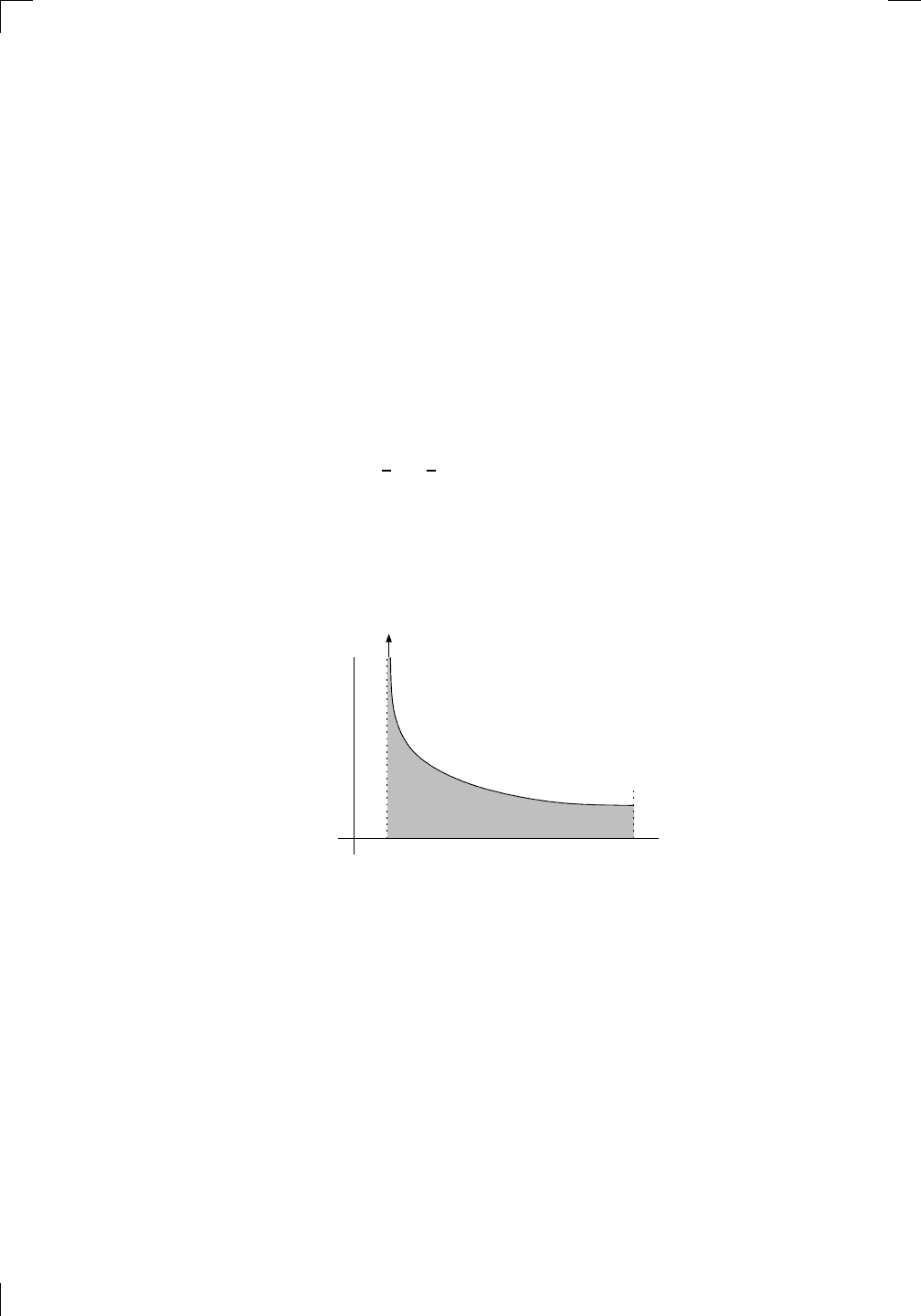
432 • Improper Integrals: Basic Concepts
There’s a different type of unboundedness that can occur even if f is
bounded. The interval [a, b] can actually be infinite—something like [0, ∞),
[−7, ∞), (−∞, 3] or even (−∞, ∞). This also makes the above integral im-
proper.
So, the integral
R
b
a
f(x) dx is improper if any of the following conditions
apply:
1. f isn’t bounded in the closed interval [a, b];
2. b = ∞; or
3. a = −∞.
For now, let’s concentrate on what happens if the first of these conditions
fails; we’ll return to the other two conditions in Section 20.2 below. As I said,
the typical way that a function fails to be unbounded is if it has a vertical
asymptote somewhere, although there can be more exotic types of behavior.
(An example is f (x) =
1
x
sin(
1
x
), which oscillates really wildly as x approaches
0.) If f(x) is unbounded for x near some number c, we’ll say that f has a
blow-up point at x = c. Again, in most situations, this is the same thing as a
vertical asymptote.
So let’s look at the simple case of when our function f has a vertical
asymptote at x = a. The situation looks something like this:
PSfrag
replacements
(
a, b)
[
a, b]
(
a, b]
[
a, b)
(
a, ∞)
[
a, ∞)
(
−∞, b)
(
−∞, b]
(
−∞, ∞)
{
x : a < x < b}
{
x : a ≤ x ≤ b}
{
x : a < x ≤ b}
{
x : a ≤ x < b}
{
x : x ≥ a}
{
x : x > a}
{
x : x ≤ b}
{
x : x < b}
R
a
b
shado
w
0
1
4
−
2
3
−
3
g(
x) = x
2
f(
x) = x
3
g(
x) = x
2
f(
x) = x
3
mirror
(y = x)
f
−
1
(x) =
3
√
x
y = h
(x)
y = h
−
1
(x)
y =
(x − 1)
2
−
1
x
Same
height
−
x
Same
length,
opp
osite signs
y = −
2x
−
2
1
y =
1
2
x − 1
2
−
1
y =
2
x
y =
10
x
y =
2
−x
y =
log
2
(x)
4
3
units
mirror
(x-axis)
y = |
x|
y = |
log
2
(x)|
θ radians
θ units
30
◦
=
π
6
45
◦
=
π
4
60
◦
=
π
3
120
◦
=
2
π
3
135
◦
=
3
π
4
150
◦
=
5
π
6
90
◦
=
π
2
180
◦
= π
210
◦
=
7
π
6
225
◦
=
5
π
4
240
◦
=
4
π
3
270
◦
=
3
π
2
300
◦
=
5
π
3
315
◦
=
7
π
4
330
◦
=
11
π
6
0
◦
=
0 radians
θ
hypotenuse
opp
osite
adjacen
t
0
(≡ 2π)
π
2
π
3
π
2
I
I
I
I
II
IV
θ
(
x, y)
x
y
r
7
π
6
reference
angle
reference
angle =
π
6
sin
+
sin −
cos
+
cos −
tan
+
tan −
A
S
T
C
7
π
4
9
π
13
5
π
6
(this
angle is
5π
6
clo
ckwise)
1
2
1
2
3
4
5
6
0
−
1
−
2
−
3
−
4
−
5
−
6
−
3π
−
5
π
2
−
2π
−
3
π
2
−
π
−
π
2
3
π
3
π
5
π
2
2
π
3
π
2
π
π
2
y =
sin(x)
1
0
−
1
−
3π
−
5
π
2
−
2π
−
3
π
2
−
π
−
π
2
3
π
5
π
2
2
π
2
π
3
π
2
π
π
2
y =
sin(x)
y =
cos(x)
−
π
2
π
2
y =
tan(x), −
π
2
<
x <
π
2
0
−
π
2
π
2
y =
tan(x)
−
2π
−
3π
−
5
π
2
−
3
π
2
−
π
−
π
2
π
2
3
π
3
π
5
π
2
2
π
3
π
2
π
y =
sec(x)
y =
csc(x)
y =
cot(x)
y = f (
x)
−
1
1
2
y = g(
x)
3
y = h
(x)
4
5
−
2
f(
x) =
1
x
g(
x) =
1
x
2
etc.
0
1
π
1
2
π
1
3
π
1
4
π
1
5
π
1
6
π
1
7
π
g(
x) = sin
1
x
1
0
−
1
L
10
100
200
y =
π
2
y = −
π
2
y =
tan
−1
(x)
π
2
π
y =
sin
(x)
x
,
x > 3
0
1
−
1
a
L
f(
x) = x sin (1/x)
(0 <
x < 0.3)
h
(x) = x
g(
x) = −x
a
L
lim
x
→a
+
f(x) = L
lim
x
→a
+
f(x) = ∞
lim
x
→a
+
f(x) = −∞
lim
x
→a
+
f(x) DNE
lim
x
→a
−
f(x) = L
lim
x
→a
−
f(x) = ∞
lim
x
→a
−
f(x) = −∞
lim
x
→a
−
f(x) DNE
M
}
lim
x
→a
−
f(x) = M
lim
x
→a
f(x) = L
lim
x
→a
f(x) DNE
lim
x
→∞
f(x) = L
lim
x
→∞
f(x) = ∞
lim
x
→∞
f(x) = −∞
lim
x
→∞
f(x) DNE
lim
x
→−∞
f(x) = L
lim
x
→−∞
f(x) = ∞
lim
x
→−∞
f(x) = −∞
lim
x
→−∞
f(x) DNE
lim
x →a
+
f(
x) = ∞
lim
x →a
+
f(
x) = −∞
lim
x →a
−
f(
x) = ∞
lim
x →a
−
f(
x) = −∞
lim
x →a
f(
x) = ∞
lim
x →a
f(
x) = −∞
lim
x →a
f(
x) DNE
y = f (
x)
a
y =
|
x|
x
1
−
1
y =
|
x + 2|
x +
2
1
−
1
−
2
1
2
3
4
a
a
b
y = x sin
1
x
y = x
y = −
x
a
b
c
d
C
a
b
c
d
−
1
0
1
2
3
time
y
t
u
(
t, f(t))
(
u, f(u))
time
y
t
u
y
x
(
x, f(x))
y = |
x|
(
z, f(z))
z
y = f (
x)
a
tangen
t at x = a
b
tangen
t at x = b
c
tangen
t at x = c
y = x
2
tangen
t
at x = −
1
u
v
uv
u +
∆u
v +
∆v
(
u + ∆u)(v + ∆v)
∆
u
∆
v
u
∆v
v∆
u
∆
u∆v
y = f (
x)
1
2
−
2
y = |
x
2
− 4|
y = x
2
− 4
y = −
2x + 5
y = g(
x)
1
2
3
4
5
6
7
8
9
0
−
1
−
2
−
3
−
4
−
5
−
6
y = f(
x)
3
−
3
3
−
3
0
−
1
2
easy
hard
flat
y = f
0
(
x)
3
−
3
0
−
1
2
1
−
1
y =
sin(x)
y = x
x
A
B
O
1
C
D
sin(
x)
tan(
x)
y =
sin
(x)
x
π
2
π
1
−
1
x =
0
a =
0
x
> 0
a
> 0
x
< 0
a
< 0
rest
position
+
−
y = x
2
sin
1
x
N
A
B
H
a
b
c
O
H
A
B
C
D
h
r
R
θ
1000
2000
α
β
p
h
y = g(
x) = log
b
(x)
y = f (
x) = b
x
y = e
x
5
10
1
2
3
4
0
−
1
−
2
−
3
−
4
y =
ln(x)
y =
cosh(x)
y =
sinh(x)
y =
tanh(x)
y =
sech(x)
y =
csch(x)
y =
coth(x)
1
−
1
y = f (
x)
original
function
in
verse function
slop
e = 0 at (x, y)
slop
e is infinite at (y, x)
−
108
2
5
1
2
1
2
3
4
5
6
0
−
1
−
2
−
3
−
4
−
5
−
6
−
3π
−
5
π
2
−
2π
−
3
π
2
−
π
−
π
2
3
π
3
π
5
π
2
2
π
3
π
2
π
π
2
y =
sin(x)
1
0
−
1
−
3π
−
5
π
2
−
2π
−
3
π
2
−
π
−
π
2
3
π
5
π
2
2
π
2
π
3
π
2
π
π
2
y =
sin(x)
y =
sin(x), −
π
2
≤ x ≤
π
2
−
2
−
1
0
2
π
2
−
π
2
y =
sin
−1
(x)
y =
cos(x)
π
π
2
y =
cos
−1
(x)
−
π
2
1
x
α
β
y =
tan(x)
y =
tan(x)
1
y =
tan
−1
(x)
y =
sec(x)
y =
sec
−1
(x)
y =
csc
−1
(x)
y =
cot
−1
(x)
1
y =
cosh
−1
(x)
y =
sinh
−1
(x)
y =
tanh
−1
(x)
y =
sech
−1
(x)
y =
csch
−1
(x)
y =
coth
−1
(x)
(0
, 3)
(2
, −1)
(5
, 2)
(7
, 0)
(
−1, 44)
(0
, 1)
(1
, −12)
(2
, 305)
y =
1
2
(2
, 3)
y = f (
x)
y = g(
x)
a
b
c
a
b
c
s
c
0
c
1
(
a, f(a))
(
b, f(b))
1
2
1
2
3
4
5
6
0
−
1
−
2
−
3
−
4
−
5
−
6
−
3π
−
5
π
2
−
2π
−
3
π
2
−
π
−
π
2
3
π
3
π
5
π
2
2
π
3
π
2
π
π
2
y =
sin(x)
1
0
−
1
−
3π
−
5
π
2
−
2π
−
3
π
2
−
π
−
π
2
3
π
5
π
2
2
π
2
π
3
π
2
π
π
2
c
OR
Lo
cal maximum
Lo
cal minimum
Horizon
tal point of inflection
1
e
y = f
0
(
x)
y = f(
x) = x ln(x)
−
1
e
?
y = f(
x) = x
3
y = g(
x) = x
4
x
f(
x)
−
3
−
2
−
1
0
1
2
1
2
3
4
+
−
?
1
5
6
3
f
0
(
x)
2 −
1
2
√
6
2
+
1
2
√
6
f
00
(
x)
7
8
g
00
(
x)
f
00
(
x)
0
y =
(
x − 3)(x − 1)
2
x
3
(
x + 2)
y = x ln
(x)
1
e
−
1
e
5
−
108
2
α
β
2 −
1
2
√
6
2
+
1
2
√
6
y = x
2
(
x − 5)
3
−
e
−
1/2
√
3
e
−
1/2
√
3
−
e
−3/2
e
−
3/2
−
1
√
3
1
√
3
−
1
1
y = xe
−
3x
2
/2
y =
x
3
− 6
x
2
+ 13x − 8
x
28
2
600
500
400
300
200
100
0
−
100
−
200
−
300
−
400
−
500
−
600
0
10
−
10
5
−
5
20
−
20
15
−
15
0
4
5
6
x
P
0
(
x)
+
−
−
existing
fence
new
fence
enclosure
A
h
b
H
99
100
101
h
dA/dh
r
h
1
2
7
shallo
w
deep
LAND
SEA
N
y
z
s
t
3
11
9
L
(11)
√
11
y = L
(x)
y = f(
x)
11
y = L
(x)
y = f (
x)
F
P
a
a +
∆x
f(
a + ∆x)
L
(a + ∆x)
f(
a)
error
d
f
∆
x
a
b
y = f (
x)
true
zero
starting
approximation
b
etter approximation
v
t
3
5
50
40
60
4
20
30
25
t
1
t
2
t
3
t
4
t
n
−2
t
n
−1
t
0
= a
t
n
= b
v
1
v
2
v
3
v
4
v
n
−1
v
n
−
30
6
30
|
v|
a
b
p
q
c
v(
c)
v(
c
1
)
v(
c
2
)
v(
c
3
)
v(
c
4
)
v(
c
5
)
v(
c
6
)
t
1
t
2
t
3
t
4
t
5
c
1
c
2
c
3
c
4
c
5
c
6
t
0
=
a
t
6
=
b
t
16
=
b
t
10
=
b
a
b
x
y
y = f (
x)
1
2
y = x
5
0
−
2
y =
1
a
b
y =
sin(x)
π
−
π
0
−
1
−
2
0
2
4
y = x
2
0
1
2
3
4
2
n
4
n
6
n
2(
n−2)
n
2(
n−1)
n
2
n
n
=
2
width
of each interval =
2
n
−
2
1
3
0
I
I
I
I
II
IV
4
y
dx
y = −
x
2
− 2x + 3
3
−
5
y = |−
x
2
− 2x + 3|
I
I
I
I
Ia
5
3
0
1
2
a
b
y = f (
x)
y = g(
x)
y = x
2
a
b
5
3
0
1
2
y =
√
x
2
√
2
2
2
dy
x
2
a
b
y = f (
x)
y = g(
x)
M
m
1
2
−1
−2
0
y = e
−x
2
1
2
e
−1/4
f
av
y = f
av
c
A
M
0
1
2
a
b
x
t
y = f(t)
F (x )
y = f(t)
F (x + h )
x + h
F (x + h) − F (x)
f(x)
1
2
y = sin(x)
π
−π
−1
−2
y =
1
x
y = x
2
1
2
1
−1
y = ln|x|
θ
a
x
a
x
p
a
2
− x
2
3
x
p
9 − x
2
p
x
2
+ a
2
x
a
p
x
2
+ 15
x
√
15
x
p
x
2
− a
2
a
x
p
x
2
− 4
2
x
−
p
x
2
− a
2
a
x
−
p
x
2
− 4
2
y = f (x)
a b
I’d be lying through my teeth if I claimed that
R
b
a
f(x) dx is the area (in square
units) of the shaded region. The problem is that the region actually extends
up the page, then past the top of the page, going on and on forever, as the
arrow is trying to indicate. The region does get skinnier as it goes up, though,
because of the vertical asymptote.
Since the region never stops going up, surely its area should be infinite,
right? Not necessarily. A mathematical miracle can occur if the region is
skinny enough, and the area can actually be finite. To see how a region can
be unbounded yet have a finite area, we’ll use limits once again. Here’s the
idea: let ε be a small positive number; then you can integrate f over the
region [a + ε, b], since f is bounded there. You’ll get some nice finite number.
Now, replay the situation but with an even smaller ε. You get a new finite
number. The situation now looks something like this:
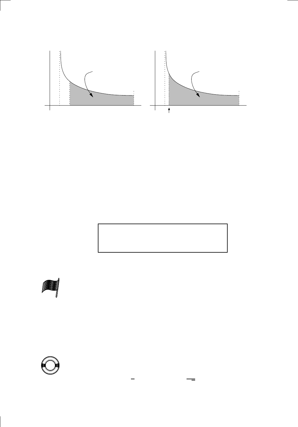
Section 20.1.1: Some examples of improper integrals • 433
PSfrag
replacements
(
a, b)
[
a, b]
(
a, b]
[
a, b)
(
a, ∞)
[
a, ∞)
(
−∞, b)
(
−∞, b]
(
−∞, ∞)
{
x : a < x < b}
{
x : a ≤ x ≤ b}
{
x : a < x ≤ b}
{
x : a ≤ x < b}
{
x : x ≥ a}
{
x : x > a}
{
x : x ≤ b}
{
x : x < b}
R
a
b
shado
w
0
1
4
−
2
3
−
3
g(
x) = x
2
f(
x) = x
3
g(
x) = x
2
f(
x) = x
3
mirror
(y = x)
f
−
1
(x) =
3
√
x
y = h
(x)
y = h
−
1
(x)
y =
(x − 1)
2
−
1
x
Same
height
−
x
Same
length,
opp
osite signs
y = −
2x
−
2
1
y =
1
2
x − 1
2
−
1
y =
2
x
y =
10
x
y =
2
−x
y =
log
2
(x)
4
3
units
mirror
(x-axis)
y = |
x|
y = |
log
2
(x)|
θ radians
θ units
30
◦
=
π
6
45
◦
=
π
4
60
◦
=
π
3
120
◦
=
2
π
3
135
◦
=
3
π
4
150
◦
=
5
π
6
90
◦
=
π
2
180
◦
= π
210
◦
=
7
π
6
225
◦
=
5
π
4
240
◦
=
4
π
3
270
◦
=
3
π
2
300
◦
=
5
π
3
315
◦
=
7
π
4
330
◦
=
11
π
6
0
◦
=
0 radians
θ
hypotenuse
opp
osite
adjacen
t
0
(≡ 2π)
π
2
π
3
π
2
I
I
I
I
II
IV
θ
(
x, y)
x
y
r
7
π
6
reference
angle
reference
angle =
π
6
sin
+
sin −
cos
+
cos −
tan
+
tan −
A
S
T
C
7
π
4
9
π
13
5
π
6
(this
angle is
5π
6
clo
ckwise)
1
2
1
2
3
4
5
6
0
−
1
−
2
−
3
−
4
−
5
−
6
−
3π
−
5
π
2
−
2π
−
3
π
2
−
π
−
π
2
3
π
3
π
5
π
2
2
π
3
π
2
π
π
2
y =
sin(x)
1
0
−
1
−
3π
−
5
π
2
−
2π
−
3
π
2
−
π
−
π
2
3
π
5
π
2
2
π
2
π
3
π
2
π
π
2
y =
sin(x)
y =
cos(x)
−
π
2
π
2
y =
tan(x), −
π
2
<
x <
π
2
0
−
π
2
π
2
y =
tan(x)
−
2π
−
3π
−
5
π
2
−
3
π
2
−
π
−
π
2
π
2
3
π
3
π
5
π
2
2
π
3
π
2
π
y =
sec(x)
y =
csc(x)
y =
cot(x)
y = f(
x)
−
1
1
2
y = g(
x)
3
y = h
(x)
4
5
−
2
f(
x) =
1
x
g(
x) =
1
x
2
etc.
0
1
π
1
2
π
1
3
π
1
4
π
1
5
π
1
6
π
1
7
π
g(
x) = sin
1
x
1
0
−
1
L
10
100
200
y =
π
2
y = −
π
2
y =
tan
−1
(x)
π
2
π
y =
sin(
x)
x
,
x > 3
0
1
−
1
a
L
f(
x) = x sin (1/x)
(0 <
x < 0.3)
h
(x) = x
g(
x) = −x
a
L
lim
x
→a
+
f(x) = L
lim
x
→a
+
f(x) = ∞
lim
x
→a
+
f(x) = −∞
lim
x
→a
+
f(x) DNE
lim
x
→a
−
f(x) = L
lim
x
→a
−
f(x) = ∞
lim
x
→a
−
f(x) = −∞
lim
x
→a
−
f(x) DNE
M
}
lim
x
→a
−
f(x) = M
lim
x
→a
f(x) = L
lim
x
→a
f(x) DNE
lim
x
→∞
f(x) = L
lim
x
→∞
f(x) = ∞
lim
x
→∞
f(x) = −∞
lim
x
→∞
f(x) DNE
lim
x
→−∞
f(x) = L
lim
x
→−∞
f(x) = ∞
lim
x
→−∞
f(x) = −∞
lim
x
→−∞
f(x) DNE
lim
x →a
+
f(
x) = ∞
lim
x →a
+
f(
x) = −∞
lim
x →a
−
f(
x) = ∞
lim
x →a
−
f(
x) = −∞
lim
x →a
f(
x) = ∞
lim
x →a
f(
x) = −∞
lim
x →a
f(
x) DNE
y = f (
x)
a
y =
|
x|
x
1
−
1
y =
|
x + 2|
x +
2
1
−
1
−
2
1
2
3
4
a
a
b
y = x sin
1
x
y = x
y = −
x
a
b
c
d
C
a
b
c
d
−
1
0
1
2
3
time
y
t
u
(
t, f (t))
(
u, f (u))
time
y
t
u
y
x
(
x, f (x))
y = |
x|
(
z, f(z))
z
y = f(
x)
a
tangen
t at x = a
b
tangen
t at x = b
c
tangen
t at x = c
y = x
2
tangen
t
at x = −
1
u
v
uv
u +
∆u
v +
∆v
(
u + ∆u)(v + ∆v)
∆
u
∆
v
u
∆v
v∆
u
∆
u∆v
y = f(
x)
1
2
−
2
y = |
x
2
− 4|
y = x
2
− 4
y = −
2x + 5
y = g(
x)
1
2
3
4
5
6
7
8
9
0
−
1
−
2
−
3
−
4
−
5
−
6
y = f (
x)
3
−
3
3
−
3
0
−
1
2
easy
hard
flat
y = f
0
(
x)
3
−
3
0
−
1
2
1
−
1
y =
sin(x)
y = x
x
A
B
O
1
C
D
sin(
x)
tan(
x)
y =
sin
(x)
x
π
2
π
1
−
1
x =
0
a =
0
x
> 0
a
> 0
x
< 0
a
< 0
rest
position
+
−
y = x
2
sin
1
x
N
A
B
H
a
b
c
O
H
A
B
C
D
h
r
R
θ
1000
2000
α
β
p
h
y = g(
x) = log
b
(x)
y = f(
x) = b
x
y = e
x
5
10
1
2
3
4
0
−
1
−
2
−
3
−
4
y =
ln(x)
y =
cosh(x)
y =
sinh(x)
y =
tanh(x)
y =
sech(x)
y =
csch(x)
y =
coth(x)
1
−
1
y = f(
x)
original
function
in
verse function
slop
e = 0 at (x, y)
slop
e is infinite at (y, x)
−
108
2
5
1
2
1
2
3
4
5
6
0
−
1
−
2
−
3
−
4
−
5
−
6
−
3π
−
5
π
2
−
2π
−
3
π
2
−
π
−
π
2
3
π
3
π
5
π
2
2
π
3
π
2
π
π
2
y =
sin(x)
1
0
−
1
−
3π
−
5
π
2
−
2π
−
3
π
2
−
π
−
π
2
3
π
5
π
2
2
π
2
π
3
π
2
π
π
2
y =
sin(x)
y =
sin(x), −
π
2
≤ x ≤
π
2
−
2
−
1
0
2
π
2
−
π
2
y =
sin
−1
(x)
y =
cos(x)
π
π
2
y =
cos
−1
(x)
−
π
2
1
x
α
β
y =
tan(x)
y =
tan(x)
1
y =
tan
−1
(x)
y =
sec(x)
y =
sec
−1
(x)
y =
csc
−1
(x)
y =
cot
−1
(x)
1
y =
cosh
−1
(x)
y =
sinh
−1
(x)
y =
tanh
−1
(x)
y =
sech
−1
(x)
y =
csch
−1
(x)
y =
coth
−1
(x)
(0
, 3)
(2
, −1)
(5
, 2)
(7
, 0)
(
−1, 44)
(0
, 1)
(1
, −12)
(2
, 305)
y =
1
2
(2
, 3)
y = f(
x)
y = g(
x)
a
b
c
a
b
c
s
c
0
c
1
(
a, f (a))
(
b, f (b))
1
2
1
2
3
4
5
6
0
−
1
−
2
−
3
−
4
−
5
−
6
−
3π
−
5
π
2
−
2π
−
3
π
2
−
π
−
π
2
3
π
3
π
5
π
2
2
π
3
π
2
π
π
2
y =
sin(x)
1
0
−
1
−
3π
−
5
π
2
−
2π
−
3
π
2
−
π
−
π
2
3
π
5
π
2
2
π
2
π
3
π
2
π
π
2
c
OR
Lo
cal maximum
Lo
cal minimum
Horizon
tal point of inflection
1
e
y = f
0
(
x)
y = f (
x) = x ln(x)
−
1
e
?
y = f (
x) = x
3
y = g(
x) = x
4
x
f(
x)
−
3
−
2
−
1
0
1
2
1
2
3
4
+
−
?
1
5
6
3
f
0
(
x)
2 −
1
2
√
6
2
+
1
2
√
6
f
00
(
x)
7
8
g
00
(
x)
f
00
(
x)
0
y =
(
x − 3)(x − 1)
2
x
3
(
x + 2)
y = x ln
(x)
1
e
−
1
e
5
−
108
2
α
β
2 −
1
2
√
6
2
+
1
2
√
6
y = x
2
(
x − 5)
3
−
e
−
1/2
√
3
e
−
1/2
√
3
−
e
−3/2
e
−
3/2
−
1
√
3
1
√
3
−
1
1
y = xe
−
3x
2
/2
y =
x
3
− 6
x
2
+ 13x − 8
x
28
2
600
500
400
300
200
100
0
−
100
−
200
−
300
−
400
−
500
−
600
0
10
−
10
5
−
5
20
−
20
15
−
15
0
4
5
6
x
P
0
(
x)
+
−
−
existing
fence
new
fence
enclosure
A
h
b
H
99
100
101
h
dA/dh
r
h
1
2
7
shallo
w
deep
LAND
SEA
N
y
z
s
t
3
11
9
L
(11)
√
11
y = L
(x)
y = f (
x)
11
y = L
(x)
y = f(
x)
F
P
a
a +
∆x
f(
a + ∆x)
L
(a + ∆x)
f(
a)
error
d
f
∆
x
a
b
y = f(
x)
true
zero
starting
approximation
b
etter approximation
v
t
3
5
50
40
60
4
20
30
25
t
1
t
2
t
3
t
4
t
n
−2
t
n
−1
t
0
= a
t
n
= b
v
1
v
2
v
3
v
4
v
n
−1
v
n
−
30
6
30
|
v|
a
b
p
q
c
v(
c)
v(
c
1
)
v(
c
2
)
v(
c
3
)
v(
c
4
)
v(
c
5
)
v(
c
6
)
t
1
t
2
t
3
t
4
t
5
c
1
c
2
c
3
c
4
c
5
c
6
t
0
=
a
t
6
=
b
t
16
=
b
t
10
=
b
a
b
x
y
y = f(
x)
1
2
y = x
5
0
−
2
y =
1
a
b
y =
sin(x)
π
−
π
0
−
1
−
2
0
2
4
y = x
2
0
1
2
3
4
2
n
4
n
6
n
2(
n−2)
n
2(
n−1)
n
2
n
n
=
2
width
of each interval =
2
n
−
2
1
3
0
I
I
I
I
II
IV
4
y
dx
y = −
x
2
− 2x + 3
3
−
5
y = |−
x
2
− 2x + 3|
I
I
I
I
Ia
5
3
0
1
2
a
b
y = f(
x)
y = g(
x)
y = x
2
a
b
5
3
0
1
2
y =
√
x
2
√
2
2
2
dy
x
2
a
b
y = f(
x)
y = g(
x)
M
m
1
2
−
1
−
2
0
y = e
−
x
2
1
2
e
−
1/4
f
a
v
y = f
a
v
c
A
M
0
1
2
a
b
x
t
y = f(t)
F (x)
y = f (t)
F (x + h )
x + h
F (x + h) − F (x)
f(x)
1
2
y = sin(x)
π
−π
−1
−2
y =
1
x
y = x
2
1
2
1
−1
y = ln|x|
θ
a
x
a
x
p
a
2
− x
2
3
x
p
9 − x
2
p
x
2
+ a
2
x
a
p
x
2
+ 15
x
√
15
x
p
x
2
− a
2
a
x
p
x
2
− 4
2
x
−
p
x
2
− a
2
a
x
−
p
x
2
− 4
2
y = f(x)
a a bb
a + ε
a + ε
εε
Z
b
a+ε
f(x) dx
Z
b
a+ε
f(x) dx
small even smaller
The smaller ε is, the closer our (bounded) approximating region is to the
actual unbounded region. This suggests that we should continue the process
with smaller and smaller ε, and see if the numbers we get have a limit L as
ε → 0
+
. If so, then we interpret L square units to be the value of the area
we’re looking for. In that case, we say that the integral
R
b
a
f(x) dx converges
to L. If there’s no limit, then we can’t find a meaningful answer for the area,
so we give up and say that the above integral diverges. Note that if the
integral isn’t improper, it automatically converges! In practice, this
means that if your function is bounded and the region of integration [a, b]
is bounded, then there’s no issue: the integral converges since it’s not even
improper. It’s just some nice finite number, no sweat.
Now, here’s a summary of the situation when you have a blow-up point at
x = a:
if f(x) is unbounded for x near a only, then set
Z
b
a
f(x) dx = lim
ε→0
+
Z
b
a+ε
f(x) dx,
provided that the limit exists. If it does, then the integral converges; if not,
the integral diverges. Just like any limit, the above one may fail to exist
because it might be ∞ or −∞, or things might oscillate around too much as
ε tends to 0
+
.
This brings us to an important point. When we look at an improper
PSfrag
replacements
(
a, b)
[
a, b]
(
a, b]
[
a, b)
(
a, ∞)
[
a, ∞)
(
−∞, b)
(
−∞, b]
(
−∞, ∞)
{
x : a < x < b}
{
x : a ≤ x ≤ b}
{
x : a < x ≤ b}
{
x : a ≤ x < b}
{
x : x ≥ a}
{
x : x > a}
{
x : x ≤ b}
{
x : x < b}
R
a
b
shado
w
0
1
4
−
2
3
−
3
g(
x) = x
2
f(
x) = x
3
g(
x) = x
2
f(
x) = x
3
mirror
(y = x)
f
−
1
(x) =
3
√
x
y = h
(x)
y = h
−
1
(x)
y =
(x − 1)
2
−
1
x
Same
height
−
x
Same
length,
opp
osite signs
y = −
2x
−
2
1
y =
1
2
x − 1
2
−
1
y =
2
x
y =
10
x
y =
2
−x
y =
log
2
(x)
4
3
units
mirror
(x-axis)
y = |
x|
y = |
log
2
(x)|
θ radians
θ units
30
◦
=
π
6
45
◦
=
π
4
60
◦
=
π
3
120
◦
=
2
π
3
135
◦
=
3
π
4
150
◦
=
5
π
6
90
◦
=
π
2
180
◦
= π
210
◦
=
7
π
6
225
◦
=
5
π
4
240
◦
=
4
π
3
270
◦
=
3
π
2
300
◦
=
5
π
3
315
◦
=
7
π
4
330
◦
=
11
π
6
0
◦
=
0 radians
θ
hypotenuse
opp
osite
adjacen
t
0
(≡ 2π)
π
2
π
3
π
2
I
I
I
I
II
IV
θ
(
x, y)
x
y
r
7
π
6
reference
angle
reference
angle =
π
6
sin
+
sin −
cos
+
cos −
tan
+
tan −
A
S
T
C
7
π
4
9
π
13
5
π
6
(this
angle is
5π
6
clo
ckwise)
1
2
1
2
3
4
5
6
0
−
1
−
2
−
3
−
4
−
5
−
6
−
3π
−
5
π
2
−
2π
−
3
π
2
−
π
−
π
2
3
π
3
π
5
π
2
2
π
3
π
2
π
π
2
y =
sin(x)
1
0
−
1
−
3π
−
5
π
2
−
2π
−
3
π
2
−
π
−
π
2
3
π
5
π
2
2
π
2
π
3
π
2
π
π
2
y =
sin(x)
y =
cos(x)
−
π
2
π
2
y =
tan(x), −
π
2
<
x <
π
2
0
−
π
2
π
2
y =
tan(x)
−
2π
−
3π
−
5
π
2
−
3
π
2
−
π
−
π
2
π
2
3
π
3
π
5
π
2
2
π
3
π
2
π
y =
sec(x)
y =
csc(x)
y =
cot(x)
y = f (
x)
−
1
1
2
y = g(
x)
3
y = h
(x)
4
5
−
2
f(
x) =
1
x
g(
x) =
1
x
2
etc.
0
1
π
1
2
π
1
3
π
1
4
π
1
5
π
1
6
π
1
7
π
g(
x) = sin
1
x
1
0
−
1
L
10
100
200
y =
π
2
y = −
π
2
y =
tan
−1
(x)
π
2
π
y =
sin(
x)
x
,
x > 3
0
1
−
1
a
L
f(
x) = x sin (1/x)
(0 <
x < 0.3)
h
(x) = x
g(
x) = −x
a
L
lim
x
→a
+
f(x) = L
lim
x
→a
+
f(x) = ∞
lim
x
→a
+
f(x) = −∞
lim
x
→a
+
f(x) DNE
lim
x
→a
−
f(x) = L
lim
x
→a
−
f(x) = ∞
lim
x
→a
−
f(x) = −∞
lim
x
→a
−
f(x) DNE
M
}
lim
x
→a
−
f(x) = M
lim
x
→a
f(x) = L
lim
x
→a
f(x) DNE
lim
x
→∞
f(x) = L
lim
x
→∞
f(x) = ∞
lim
x
→∞
f(x) = −∞
lim
x
→∞
f(x) DNE
lim
x
→−∞
f(x) = L
lim
x
→−∞
f(x) = ∞
lim
x
→−∞
f(x) = −∞
lim
x
→−∞
f(x) DNE
lim
x →a
+
f(
x) = ∞
lim
x →a
+
f(
x) = −∞
lim
x →a
−
f(
x) = ∞
lim
x →a
−
f(
x) = −∞
lim
x →a
f(
x) = ∞
lim
x →a
f(
x) = −∞
lim
x →a
f(
x) DNE
y = f (
x)
a
y =
|
x|
x
1
−
1
y =
|
x + 2|
x +
2
1
−
1
−
2
1
2
3
4
a
a
b
y = x sin
1
x
y = x
y = −
x
a
b
c
d
C
a
b
c
d
−
1
0
1
2
3
time
y
t
u
(
t, f(t))
(
u, f(u))
time
y
t
u
y
x
(
x, f(x))
y = |
x|
(
z, f(z))
z
y = f (
x)
a
tangen
t at x = a
b
tangen
t at x = b
c
tangen
t at x = c
y = x
2
tangen
t
at x = −
1
u
v
uv
u +
∆u
v +
∆v
(
u + ∆u)(v + ∆v)
∆
u
∆
v
u
∆v
v∆
u
∆
u∆v
y = f (
x)
1
2
−
2
y = |
x
2
− 4|
y = x
2
− 4
y = −
2x + 5
y = g(
x)
1
2
3
4
5
6
7
8
9
0
−
1
−
2
−
3
−
4
−
5
−
6
y = f (
x)
3
−
3
3
−
3
0
−
1
2
easy
hard
flat
y = f
0
(
x)
3
−
3
0
−
1
2
1
−
1
y =
sin(x)
y = x
x
A
B
O
1
C
D
sin(
x)
tan(
x)
y =
sin
(x)
x
π
2
π
1
−
1
x =
0
a =
0
x
> 0
a
> 0
x
< 0
a
< 0
rest
position
+
−
y = x
2
sin
1
x
N
A
B
H
a
b
c
O
H
A
B
C
D
h
r
R
θ
1000
2000
α
β
p
h
y = g(
x) = log
b
(x)
y = f (
x) = b
x
y = e
x
5
10
1
2
3
4
0
−
1
−
2
−
3
−
4
y =
ln(x)
y =
cosh(x)
y =
sinh(x)
y =
tanh(x)
y =
sech(x)
y =
csch(x)
y =
coth(x)
1
−
1
y = f (
x)
original
function
in
verse function
slop
e = 0 at (x, y)
slop
e is infinite at (y, x)
−
108
2
5
1
2
1
2
3
4
5
6
0
−
1
−
2
−
3
−
4
−
5
−
6
−
3π
−
5
π
2
−
2π
−
3
π
2
−
π
−
π
2
3
π
3
π
5
π
2
2
π
3
π
2
π
π
2
y =
sin(x)
1
0
−
1
−
3π
−
5
π
2
−
2π
−
3
π
2
−
π
−
π
2
3
π
5
π
2
2
π
2
π
3
π
2
π
π
2
y =
sin(x)
y =
sin(x), −
π
2
≤ x ≤
π
2
−
2
−
1
0
2
π
2
−
π
2
y =
sin
−1
(x)
y =
cos(x)
π
π
2
y =
cos
−1
(x)
−
π
2
1
x
α
β
y =
tan(x)
y =
tan(x)
1
y =
tan
−1
(x)
y =
sec(x)
y =
sec
−1
(x)
y =
csc
−1
(x)
y =
cot
−1
(x)
1
y =
cosh
−1
(x)
y =
sinh
−1
(x)
y =
tanh
−1
(x)
y =
sech
−1
(x)
y =
csch
−1
(x)
y =
coth
−1
(x)
(0
, 3)
(2
, −1)
(5
, 2)
(7
, 0)
(
−1, 44)
(0
, 1)
(1
, −12)
(2
, 305)
y =
1
2
(2
, 3)
y = f (
x)
y = g(
x)
a
b
c
a
b
c
s
c
0
c
1
(
a, f(a))
(
b, f(b))
1
2
1
2
3
4
5
6
0
−
1
−
2
−
3
−
4
−
5
−
6
−
3π
−
5
π
2
−
2π
−
3
π
2
−
π
−
π
2
3
π
3
π
5
π
2
2
π
3
π
2
π
π
2
y =
sin(x)
1
0
−
1
−
3π
−
5
π
2
−
2π
−
3
π
2
−
π
−
π
2
3
π
5
π
2
2
π
2
π
3
π
2
π
π
2
c
OR
Lo
cal maximum
Lo
cal minimum
Horizon
tal point of inflection
1
e
y = f
0
(
x)
y = f(
x) = x ln(x)
−
1
e
?
y = f(
x) = x
3
y = g(
x) = x
4
x
f(
x)
−
3
−
2
−
1
0
1
2
1
2
3
4
+
−
?
1
5
6
3
f
0
(
x)
2 −
1
2
√
6
2
+
1
2
√
6
f
00
(
x)
7
8
g
00
(
x)
f
00
(
x)
0
y =
(
x − 3)(x − 1)
2
x
3
(
x + 2)
y = x ln
(x)
1
e
−
1
e
5
−
108
2
α
β
2 −
1
2
√
6
2
+
1
2
√
6
y = x
2
(
x − 5)
3
−
e
−
1/2
√
3
e
−
1/2
√
3
−
e
−3/2
e
−
3/2
−
1
√
3
1
√
3
−
1
1
y = xe
−
3x
2
/2
y =
x
3
− 6
x
2
+ 13x − 8
x
28
2
600
500
400
300
200
100
0
−
100
−
200
−
300
−
400
−
500
−
600
0
10
−
10
5
−
5
20
−
20
15
−
15
0
4
5
6
x
P
0
(
x)
+
−
−
existing
fence
new
fence
enclosure
A
h
b
H
99
100
101
h
dA/dh
r
h
1
2
7
shallo
w
deep
LAND
SEA
N
y
z
s
t
3
11
9
L
(11)
√
11
y = L
(x)
y = f (
x)
11
y = L
(x)
y = f (
x)
F
P
a
a +
∆x
f(
a + ∆x)
L
(a + ∆x)
f(
a)
error
d
f
∆
x
a
b
y = f (
x)
true
zero
starting
approximation
b
etter approximation
v
t
3
5
50
40
60
4
20
30
25
t
1
t
2
t
3
t
4
t
n
−2
t
n
−1
t
0
= a
t
n
= b
v
1
v
2
v
3
v
4
v
n
−1
v
n
−
30
6
30
|
v|
a
b
p
q
c
v(
c)
v(
c
1
)
v(
c
2
)
v(
c
3
)
v(
c
4
)
v(
c
5
)
v(
c
6
)
t
1
t
2
t
3
t
4
t
5
c
1
c
2
c
3
c
4
c
5
c
6
t
0
=
a
t
6
=
b
t
16
=
b
t
10
=
b
a
b
x
y
y = f (
x)
1
2
y = x
5
0
−
2
y =
1
a
b
y =
sin(x)
π
−
π
0
−
1
−
2
0
2
4
y = x
2
0
1
2
3
4
2
n
4
n
6
n
2(
n−2)
n
2(
n−1)
n
2
n
n
=
2
width
of each interval =
2
n
−
2
1
3
0
I
I
I
I
II
IV
4
y
dx
y = −
x
2
− 2x + 3
3
−
5
y = |−
x
2
− 2x + 3|
I
I
I
I
Ia
5
3
0
1
2
a
b
y = f (
x)
y = g(
x)
y = x
2
a
b
5
3
0
1
2
y =
√
x
2
√
2
2
2
dy
x
2
a
b
y = f (
x)
y = g(
x)
M
m
1
2
−1
−2
0
y = e
−x
2
1
2
e
−1/4
f
av
y = f
av
c
A
M
0
1
2
a
b
x
t
y = f(t)
F (x )
y = f(t)
F (x + h )
x + h
F (x + h) − F (x)
f(x)
1
2
y = sin(x)
π
−π
−1
−2
y =
1
x
y = x
2
1
2
1
−1
y = ln|x|
θ
a
x
a
x
p
a
2
− x
2
3
x
p
9 − x
2
p
x
2
+ a
2
x
a
p
x
2
+ 15
x
√
15
x
p
x
2
− a
2
a
x
p
x
2
− 4
2
x
−
p
x
2
− a
2
a
x
−
p
x
2
− 4
2
y = f (x)
a
b
a + ε
ε
Z
b
a+ε
f(x) dx
small
even smaller
integral, the most important thing we need to find out is whether it converges
or diverges. It’s much less important to know what the integral converges to
(assuming it converges). In practice, you can use computational techniques
to estimate the value, but only if you know that the integral converges. If the
integral diverges, you can get some whacked-out results if you try to use a
computer to approximate your integral. Computers don’t really understand
infinities or crazy oscillations (yet!).
20.1.1 Some examples of improper integrals
Consider the integrals
PSfrag
replacements
(
a, b)
[
a, b]
(
a, b]
[
a, b)
(
a, ∞)
[
a, ∞)
(
−∞, b)
(
−∞, b]
(
−∞, ∞)
{
x : a < x < b}
{
x : a ≤ x ≤ b}
{
x : a < x ≤ b}
{
x : a ≤ x < b}
{
x : x ≥ a}
{
x : x > a}
{
x : x ≤ b}
{
x : x < b}
R
a
b
shado
w
0
1
4
−
2
3
−
3
g(
x) = x
2
f(
x) = x
3
g(
x) = x
2
f(
x) = x
3
mirror
(y = x)
f
−
1
(x) =
3
√
x
y = h
(x)
y = h
−
1
(x)
y =
(x − 1)
2
−
1
x
Same
height
−
x
Same
length,
opp
osite signs
y = −
2x
−
2
1
y =
1
2
x − 1
2
−
1
y =
2
x
y =
10
x
y =
2
−x
y =
log
2
(x)
4
3
units
mirror
(x-axis)
y = |
x|
y = |
log
2
(x)|
θ radians
θ units
30
◦
=
π
6
45
◦
=
π
4
60
◦
=
π
3
120
◦
=
2
π
3
135
◦
=
3
π
4
150
◦
=
5
π
6
90
◦
=
π
2
180
◦
= π
210
◦
=
7
π
6
225
◦
=
5
π
4
240
◦
=
4
π
3
270
◦
=
3
π
2
300
◦
=
5
π
3
315
◦
=
7
π
4
330
◦
=
11
π
6
0
◦
=
0 radians
θ
hypotenuse
opp
osite
adjacen
t
0
(≡ 2π)
π
2
π
3
π
2
I
I
I
I
II
IV
θ
(
x, y)
x
y
r
7
π
6
reference
angle
reference
angle =
π
6
sin
+
sin −
cos
+
cos −
tan
+
tan −
A
S
T
C
7
π
4
9
π
13
5
π
6
(this
angle is
5π
6
clo
ckwise)
1
2
1
2
3
4
5
6
0
−
1
−
2
−
3
−
4
−
5
−
6
−
3π
−
5
π
2
−
2π
−
3
π
2
−
π
−
π
2
3
π
3
π
5
π
2
2
π
3
π
2
π
π
2
y =
sin(x)
1
0
−
1
−
3π
−
5
π
2
−
2π
−
3
π
2
−
π
−
π
2
3
π
5
π
2
2
π
2
π
3
π
2
π
π
2
y =
sin(x)
y =
cos(x)
−
π
2
π
2
y =
tan(x), −
π
2
<
x <
π
2
0
−
π
2
π
2
y =
tan(x)
−
2π
−
3π
−
5
π
2
−
3
π
2
−
π
−
π
2
π
2
3
π
3
π
5
π
2
2
π
3
π
2
π
y =
sec(x)
y =
csc(x)
y =
cot(x)
y = f(
x)
−
1
1
2
y = g(
x)
3
y = h
(x)
4
5
−
2
f(
x) =
1
x
g(
x) =
1
x
2
etc.
0
1
π
1
2
π
1
3
π
1
4
π
1
5
π
1
6
π
1
7
π
g(
x) = sin
1
x
1
0
−
1
L
10
100
200
y =
π
2
y = −
π
2
y =
tan
−1
(x)
π
2
π
y =
sin(
x)
x
,
x > 3
0
1
−
1
a
L
f(
x) = x sin (1/x)
(0 <
x < 0.3)
h
(x) = x
g(
x) = −x
a
L
lim
x
→a
+
f(x) = L
lim
x
→a
+
f(x) = ∞
lim
x
→a
+
f(x) = −∞
lim
x
→a
+
f(x) DNE
lim
x
→a
−
f(x) = L
lim
x
→a
−
f(x) = ∞
lim
x
→a
−
f(x) = −∞
lim
x
→a
−
f(x) DNE
M
}
lim
x
→a
−
f(x) = M
lim
x
→a
f(x) = L
lim
x
→a
f(x) DNE
lim
x
→∞
f(x) = L
lim
x
→∞
f(x) = ∞
lim
x
→∞
f(x) = −∞
lim
x
→∞
f(x) DNE
lim
x
→−∞
f(x) = L
lim
x
→−∞
f(x) = ∞
lim
x
→−∞
f(x) = −∞
lim
x
→−∞
f(x) DNE
lim
x →a
+
f(
x) = ∞
lim
x →a
+
f(
x) = −∞
lim
x →a
−
f(
x) = ∞
lim
x →a
−
f(
x) = −∞
lim
x →a
f(
x) = ∞
lim
x →a
f(
x) = −∞
lim
x →a
f(
x) DNE
y = f (
x)
a
y =
|
x|
x
1
−
1
y =
|
x + 2|
x +
2
1
−
1
−
2
1
2
3
4
a
a
b
y = x sin
1
x
y = x
y = −
x
a
b
c
d
C
a
b
c
d
−
1
0
1
2
3
time
y
t
u
(
t, f(t))
(
u, f(u))
time
y
t
u
y
x
(
x, f(x))
y = |
x|
(
z, f(z))
z
y = f(
x)
a
tangen
t at x = a
b
tangen
t at x = b
c
tangen
t at x = c
y = x
2
tangen
t
at x = −
1
u
v
uv
u +
∆u
v +
∆v
(
u + ∆u)(v + ∆v)
∆
u
∆
v
u
∆v
v∆
u
∆
u∆v
y = f(
x)
1
2
−
2
y = |
x
2
− 4|
y = x
2
− 4
y = −
2x + 5
y = g(
x)
1
2
3
4
5
6
7
8
9
0
−
1
−
2
−
3
−
4
−
5
−
6
y = f (
x)
3
−
3
3
−
3
0
−
1
2
easy
hard
flat
y = f
0
(
x)
3
−
3
0
−
1
2
1
−
1
y =
sin(x)
y = x
x
A
B
O
1
C
D
sin(
x)
tan(
x)
y =
sin(
x)
x
π
2
π
1
−
1
x =
0
a =
0
x
> 0
a
> 0
x
< 0
a
< 0
rest
position
+
−
y = x
2
sin
1
x
N
A
B
H
a
b
c
O
H
A
B
C
D
h
r
R
θ
1000
2000
α
β
p
h
y = g(
x) = log
b
(x)
y = f(
x) = b
x
y = e
x
5
10
1
2
3
4
0
−
1
−
2
−
3
−
4
y =
ln(x)
y =
cosh(x)
y =
sinh(x)
y =
tanh(x)
y =
sech(x)
y =
csch(x)
y =
coth(x)
1
−
1
y = f(
x)
original
function
in
verse function
slop
e = 0 at (x, y)
slop
e is infinite at (y, x)
−
108
2
5
1
2
1
2
3
4
5
6
0
−
1
−
2
−
3
−
4
−
5
−
6
−
3π
−
5
π
2
−
2π
−
3
π
2
−
π
−
π
2
3
π
3
π
5
π
2
2
π
3
π
2
π
π
2
y =
sin(x)
1
0
−
1
−
3π
−
5
π
2
−
2π
−
3
π
2
−
π
−
π
2
3
π
5
π
2
2
π
2
π
3
π
2
π
π
2
y =
sin(x)
y =
sin(x), −
π
2
≤ x ≤
π
2
−
2
−
1
0
2
π
2
−
π
2
y =
sin
−1
(x)
y =
cos(x)
π
π
2
y =
cos
−1
(x)
−
π
2
1
x
α
β
y =
tan(x)
y =
tan(x)
1
y =
tan
−1
(x)
y =
sec(x)
y =
sec
−1
(x)
y =
csc
−1
(x)
y =
cot
−1
(x)
1
y =
cosh
−1
(x)
y =
sinh
−1
(x)
y =
tanh
−1
(x)
y =
sech
−1
(x)
y =
csch
−1
(x)
y =
coth
−1
(x)
(0
, 3)
(2
, −1)
(5
, 2)
(7
, 0)
(
−1, 44)
(0
, 1)
(1
, −12)
(2
, 305)
y =
1
2
(2
, 3)
y = f(
x)
y = g(
x)
a
b
c
a
b
c
s
c
0
c
1
(
a, f(a))
(
b, f(b))
1
2
1
2
3
4
5
6
0
−
1
−
2
−
3
−
4
−
5
−
6
−
3π
−
5
π
2
−
2π
−
3
π
2
−
π
−
π
2
3
π
3
π
5
π
2
2
π
3
π
2
π
π
2
y =
sin(x)
1
0
−
1
−
3π
−
5
π
2
−
2π
−
3
π
2
−
π
−
π
2
3
π
5
π
2
2
π
2
π
3
π
2
π
π
2
c
OR
Lo
cal maximum
Lo
cal minimum
Horizon
tal point of inflection
1
e
y = f
0
(
x)
y = f (
x) = x ln(x)
−
1
e
?
y = f(
x) = x
3
y = g(
x) = x
4
x
f(
x)
−
3
−
2
−
1
0
1
2
1
2
3
4
+
−
?
1
5
6
3
f
0
(
x)
2 −
1
2
√
6
2
+
1
2
√
6
f
00
(
x)
7
8
g
00
(
x)
f
00
(
x)
0
y =
(
x − 3)(x − 1)
2
x
3
(
x + 2)
y = x ln
(x)
1
e
−
1
e
5
−
108
2
α
β
2 −
1
2
√
6
2
+
1
2
√
6
y = x
2
(
x − 5)
3
−
e
−
1/2
√
3
e
−
1/2
√
3
−
e
−3/2
e
−
3/2
−
1
√
3
1
√
3
−
1
1
y = xe
−
3x
2
/2
y =
x
3
− 6
x
2
+ 13x − 8
x
28
2
600
500
400
300
200
100
0
−
100
−
200
−
300
−
400
−
500
−
600
0
10
−
10
5
−
5
20
−
20
15
−
15
0
4
5
6
x
P
0
(
x)
+
−
−
existing
fence
new
fence
enclosure
A
h
b
H
99
100
101
h
dA/dh
r
h
1
2
7
shallo
w
deep
LAND
SEA
N
y
z
s
t
3
11
9
L
(11)
√
11
y = L
(x)
y = f (
x)
11
y = L
(x)
y = f(
x)
F
P
a
a +
∆x
f(
a + ∆x)
L
(a + ∆x)
f(
a)
error
d
f
∆
x
a
b
y = f(
x)
true
zero
starting
approximation
b
etter approximation
v
t
3
5
50
40
60
4
20
30
25
t
1
t
2
t
3
t
4
t
n
−2
t
n
−1
t
0
= a
t
n
= b
v
1
v
2
v
3
v
4
v
n
−1
v
n
−
30
6
30
|
v|
a
b
p
q
c
v(
c)
v(
c
1
)
v(
c
2
)
v(
c
3
)
v(
c
4
)
v(
c
5
)
v(
c
6
)
t
1
t
2
t
3
t
4
t
5
c
1
c
2
c
3
c
4
c
5
c
6
t
0
=
a
t
6
=
b
t
16
=
b
t
10
=
b
a
b
x
y
y = f(
x)
1
2
y = x
5
0
−
2
y =
1
a
b
y =
sin(x)
π
−
π
0
−
1
−
2
0
2
4
y = x
2
0
1
2
3
4
2
n
4
n
6
n
2(
n−2)
n
2(
n−1)
n
2
n
n
=
2
width
of each interval =
2
n
−
2
1
3
0
I
I
I
I
II
IV
4
y
dx
y = −
x
2
− 2x + 3
3
−
5
y = |−
x
2
− 2x + 3|
I
I
I
I
Ia
5
3
0
1
2
a
b
y = f (
x)
y = g(
x)
y = x
2
a
b
5
3
0
1
2
y =
√
x
2
√
2
2
2
dy
x
2
a
b
y = f(x)
y = g(x)
M
m
1
2
−1
−2
0
y = e
−x
2
1
2
e
−1/4
f
av
y = f
av
c
A
M
0
1
2
a
b
x
t
y = f (t)
F (x )
y = f (t)
F (x + h)
x + h
F (x + h) − F (x)
f(x)
1
2
y = sin(x)
π
−π
−1
−2
y =
1
x
y = x
2
1
2
1
−1
y = ln|x|
θ
a
x
a
x
p
a
2
− x
2
3
x
p
9 − x
2
p
x
2
+ a
2
x
a
p
x
2
+ 15
x
√
15
x
p
x
2
− a
2
a
x
p
x
2
− 4
2
x
−
p
x
2
− a
2
a
x
−
p
x
2
− 4
2
y = f(x)
a
b
a + ε
ε
Z
b
a+ε
f(x) dx
small
even smaller
Z
1
0
1
x
dx and
Z
1
0
1
√
x
dx.
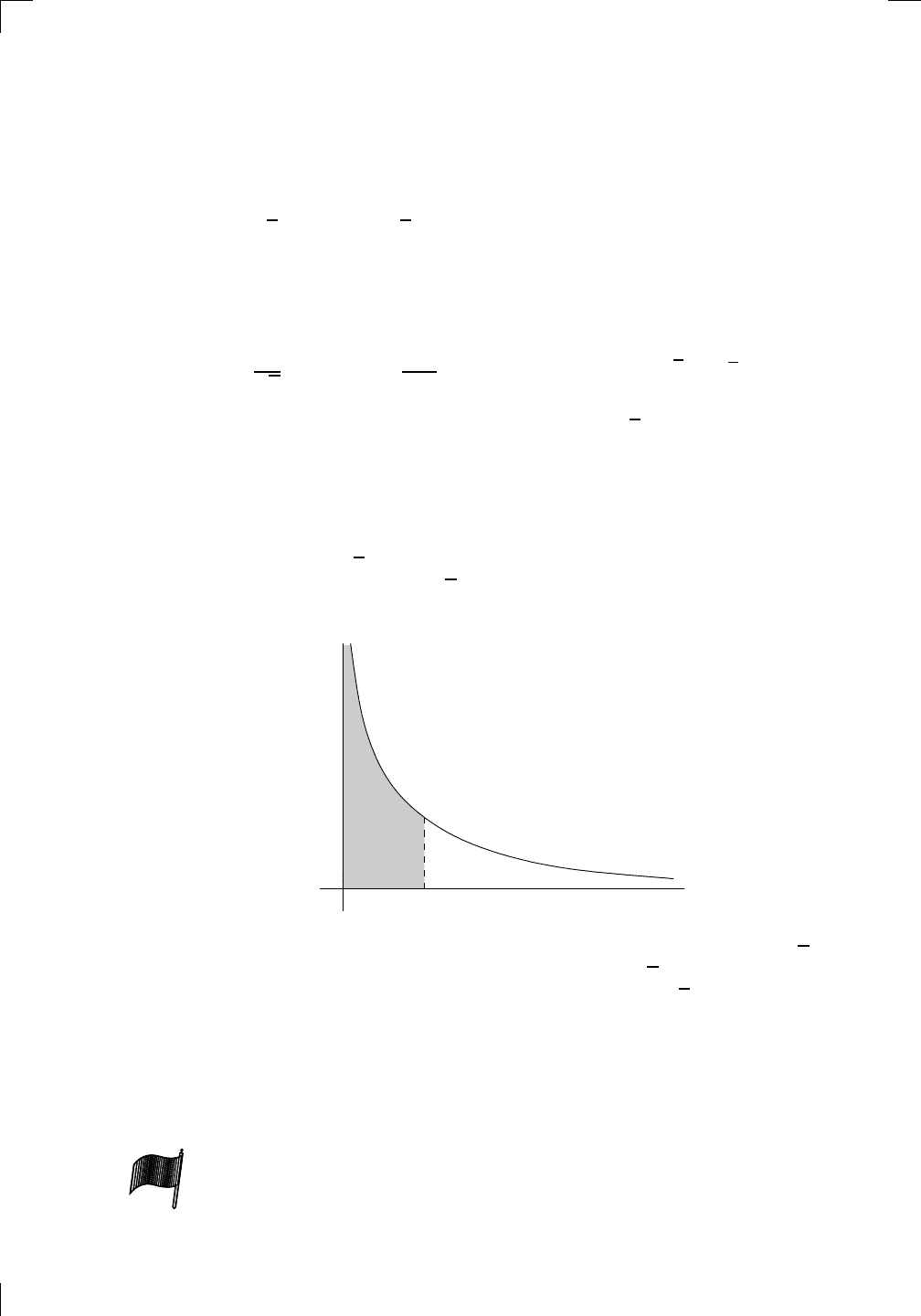
434 • Improper Integrals: Basic Concepts
These are both improper because their integrands have vertical asymptotes
at x = 0. So we’ll use the formula in the box above. In the first case, we have
Z
1
0
1
x
dx = lim
ε→0
+
Z
1
ε
1
x
dx = lim
ε→0
+
ln|x|
1
ε
= lim
ε→0
+
(ln(1) − ln(ε)) = ∞.
(We have used the facts that ln(1) = 0 and that ln(ε) → −∞ as ε → 0
+
.)
Since we got ∞, the improper integral
R
1
0
1/x dx must diverge. How about
the other integral? Using the formula again, we have
Z
1
0
1
√
x
dx = lim
ε→0
+
Z
1
ε
1
x
1/2
dx = lim
ε→0
+
2x
1/2
1
ε
= lim
ε→0
+
(2
√
1 − 2
√
ε) = 2.
We got a nice finite number, so the integral
R
1
0
1/
√
x dx converges. As it
happens, we’ve shown that the integral converges to 2, but as I said at the
end of the last section, we don’t care that much. Our main focus is to decide
whether an improper integral converges, without worrying what it actually
converges to.
What’s really going on here? Why should the improper integral
R
1
0
1/x dx
diverge but
R
1
0
1/
√
x dx converge? After all, when you think about it, the
graphs of y = 1/x and y = 1/
√
x look roughly the same—something like this:
PSfrag replacements
(
a, b)
[
a, b]
(
a, b]
[
a, b)
(
a, ∞)
[
a, ∞)
(
−∞, b)
(
−∞, b]
(
−∞, ∞)
{
x : a < x < b}
{
x : a ≤ x ≤ b}
{
x : a < x ≤ b}
{
x : a ≤ x < b}
{
x : x ≥ a}
{
x : x > a}
{
x : x ≤ b}
{
x : x < b}
R
a
b
shadow
0
1
4
−
2
3
−
3
g(
x) = x
2
f(
x) = x
3
g(
x) = x
2
f(
x) = x
3
mirror (
y = x)
f
−
1
(x) =
3
√
x
y = h
(x)
y = h
−
1
(x)
y = (
x − 1)
2
−
1
x
Same height
−
x
Same length,
opposite signs
y = −
2x
−
2
1
y =
1
2
x − 1
2
−
1
y = 2
x
y = 10
x
y = 2
−
x
y = log
2
(
x)
4
3 units
mirror (
x-axis)
y = |
x|
y = |
log
2
(x)|
θ radians
θ units
30
◦
=
π
6
45
◦
=
π
4
60
◦
=
π
3
120
◦
=
2
π
3
135
◦
=
3
π
4
150
◦
=
5
π
6
90
◦
=
π
2
180
◦
= π
210
◦
=
7
π
6
225
◦
=
5
π
4
240
◦
=
4
π
3
270
◦
=
3
π
2
300
◦
=
5
π
3
315
◦
=
7
π
4
330
◦
=
11
π
6
0
◦
= 0 radians
θ
hypotenuse
opposite
adjacent
0 (
≡ 2π)
π
2
π
3
π
2
I
II
III
IV
θ
(
x, y)
x
y
r
7
π
6
reference angle
reference angle =
π
6
sin +
sin −
cos +
cos −
tan +
tan −
A
S
T
C
7
π
4
9
π
13
5
π
6
(this angle is
5
π
6
clockwise)
1
2
1
2
3
4
5
6
0
−
1
−
2
−
3
−
4
−
5
−
6
−
3π
−
5
π
2
−
2π
−
3
π
2
−
π
−
π
2
3
π
3
π
5
π
2
2
π
3
π
2
π
π
2
y = sin(
x)
1
0
−
1
−
3π
−
5
π
2
−
2π
−
3
π
2
−
π
−
π
2
3
π
5
π
2
2
π
2
π
3
π
2
π
π
2
y = sin(
x)
y = cos(
x)
−
π
2
π
2
y = tan(
x), −
π
2
< x <
π
2
0
−
π
2
π
2
y = tan(
x)
−
2π
−
3π
−
5
π
2
−
3
π
2
−
π
−
π
2
π
2
3
π
3
π
5
π
2
2
π
3
π
2
π
y = sec(
x)
y = csc(
x)
y = cot(
x)
y = f(
x)
−
1
1
2
y = g(
x)
3
y = h
(x)
4
5
−
2
f(
x) =
1
x
g(
x) =
1
x
2
etc.
0
1
π
1
2
π
1
3
π
1
4
π
1
5
π
1
6
π
1
7
π
g(
x) = sin
1
x
1
0
−
1
L
10
100
200
y =
π
2
y = −
π
2
y = tan
−
1
(x)
π
2
π
y =
sin(
x)
x
, x > 3
0
1
−
1
a
L
f(
x) = x sin (1/x)
(0 < x < 0
.3)
h
(x) = x
g(
x) = −x
a
L
lim
x
→a
+
f(x) = L
lim
x
→a
+
f(x) = ∞
lim
x
→a
+
f(x) = −∞
lim
x
→a
+
f(x) DNE
lim
x
→a
−
f(x) = L
lim
x
→a
−
f(x) = ∞
lim
x
→a
−
f(x) = −∞
lim
x
→a
−
f(x) DNE
M
}
lim
x
→a
−
f(x) = M
lim
x
→a
f(x) = L
lim
x
→a
f(x) DNE
lim
x
→∞
f(x) = L
lim
x
→∞
f(x) = ∞
lim
x
→∞
f(x) = −∞
lim
x
→∞
f(x) DNE
lim
x
→−∞
f(x) = L
lim
x
→−∞
f(x) = ∞
lim
x
→−∞
f(x) = −∞
lim
x
→−∞
f(x) DNE
lim
x →a
+
f(
x) = ∞
lim
x →a
+
f(
x) = −∞
lim
x →a
−
f(
x) = ∞
lim
x →a
−
f(
x) = −∞
lim
x →a
f(
x) = ∞
lim
x →a
f(
x) = −∞
lim
x →a
f(
x) DNE
y = f(
x)
a
y =
|
x|
x
1
−
1
y =
|
x + 2|
x + 2
1
−
1
−
2
1
2
3
4
a
a
b
y = x sin
1
x
y = x
y = −
x
a
b
c
d
C
a
b
c
d
−
1
0
1
2
3
time
y
t
u
(
t, f(t))
(
u, f(u))
time
y
t
u
y
x
(
x, f(x))
y = |
x|
(
z, f(z))
z
y = f(
x)
a
tangent at x = a
b
tangent at x = b
c
tangent at x = c
y = x
2
tangent
at x = −
1
u
v
uv
u + ∆
u
v + ∆
v
(
u + ∆u)(v + ∆v)
∆
u
∆
v
u
∆v
v∆
u
∆
u∆v
y = f(
x)
1
2
−
2
y = |
x
2
− 4|
y = x
2
− 4
y = −
2x + 5
y = g(
x)
1
2
3
4
5
6
7
8
9
0
−
1
−
2
−
3
−
4
−
5
−
6
y = f(
x)
3
−
3
3
−
3
0
−
1
2
easy
hard
flat
y = f
0
(
x)
3
−
3
0
−
1
2
1
−
1
y = sin(
x)
y = x
x
A
B
O
1
C
D
sin(
x)
tan(
x)
y =
sin(
x)
x
π
2
π
1
−
1
x = 0
a = 0
x > 0
a > 0
x < 0
a < 0
rest position
+
−
y = x
2
sin
1
x
N
A
B
H
a
b
c
O
H
A
B
C
D
h
r
R
θ
1000
2000
α
β
p
h
y = g(
x) = log
b
(x)
y = f(
x) = b
x
y = e
x
5
10
1
2
3
4
0
−
1
−
2
−
3
−
4
y = ln(
x)
y = cosh(
x)
y = sinh(
x)
y = tanh(
x)
y = sech(
x)
y = csch(
x)
y = coth(
x)
1
−
1
y = f(
x)
original function
inverse function
slope = 0 at (
x, y)
slope is infinite at (
y, x)
−
108
2
5
1
2
1
2
3
4
5
6
0
−
1
−
2
−
3
−
4
−
5
−
6
−
3π
−
5
π
2
−
2π
−
3
π
2
−
π
−
π
2
3
π
3
π
5
π
2
2
π
3
π
2
π
π
2
y = sin(
x)
1
0
−
1
−
3π
−
5
π
2
−
2π
−
3
π
2
−
π
−
π
2
3
π
5
π
2
2
π
2
π
3
π
2
π
π
2
y = sin(
x)
y = sin(
x), −
π
2
≤ x ≤
π
2
−
2
−
1
0
2
π
2
−
π
2
y = sin
−
1
(x)
y = cos(
x)
π
π
2
y = cos
−
1
(x)
−
π
2
1
x
α
β
y = tan(
x)
y = tan(
x)
1
y = tan
−
1
(x)
y = sec(
x)
y = sec
−
1
(x)
y = csc
−
1
(x)
y = cot
−
1
(x)
1
y = cosh
−
1
(x)
y = sinh
−
1
(x)
y = tanh
−
1
(x)
y = sech
−
1
(x)
y = csch
−
1
(x)
y = coth
−
1
(x)
(0
, 3)
(2
, −1)
(5
, 2)
(7
, 0)
(
−1, 44)
(0
, 1)
(1
, −12)
(2
, 305)
y = 1
2
(2
, 3)
y = f(
x)
y = g(
x)
a
b
c
a
b
c
s
c
0
c
1
(
a, f(a))
(
b, f(b))
1
2
1
2
3
4
5
6
0
−
1
−
2
−
3
−
4
−
5
−
6
−
3π
−
5
π
2
−
2π
−
3
π
2
−
π
−
π
2
3
π
3
π
5
π
2
2
π
3
π
2
π
π
2
y = sin(
x)
1
0
−
1
−
3π
−
5
π
2
−
2π
−
3
π
2
−
π
−
π
2
3
π
5
π
2
2
π
2
π
3
π
2
π
π
2
c
OR
Local maximum
Local minimum
Horizontal point of inflection
1
e
y = f
0
(
x)
y = f(
x) = x ln(x)
−
1
e
?
y = f (
x) = x
3
y = g(
x) = x
4
x
f(
x)
−
3
−
2
−
1
0
1
2
1
2
3
4
+
−
?
1
5
6
3
f
0
(
x)
2 −
1
2
√
6
2 +
1
2
√
6
f
00
(
x)
7
8
g
00
(
x)
f
00
(
x)
0
y =
(
x − 3)(x − 1)
2
x
3
(
x + 2)
y = x ln(
x)
1
e
−
1
e
5
−
108
2
α
β
2 −
1
2
√
6
2 +
1
2
√
6
y = x
2
(
x − 5)
3
−
e
−
1/2
√
3
e
−
1/2
√
3
−
e
−3/2
e
−
3/2
−
1
√
3
1
√
3
−
1
1
y = xe
−
3x
2
/2
y =
x
3
− 6
x
2
+ 13x − 8
x
28
2
600
500
400
300
200
100
0
−
100
−
200
−
300
−
400
−
500
−
600
0
10
−
10
5
−
5
20
−
20
15
−
15
0
4
5
6
x
P
0
(
x)
+
−
−
existing fence
new fence
enclosure
A
h
b
H
99
100
101
h
dA/dh
r
h
1
2
7
shallow
deep
LAND
SEA
N
y
z
s
t
3
11
9
L
(11)
√
11
y = L
(x)
y = f(
x)
11
y = L
(x)
y = f(
x)
F
P
a
a + ∆
x
f(
a + ∆x)
L
(a + ∆x)
f(
a)
error
df
∆
x
a
b
y = f(
x)
true zero
starting approximation
better approximation
v
t
3
5
50
40
60
4
20
30
25
t
1
t
2
t
3
t
4
t
n
−2
t
n
−1
t
0
= a
t
n
= b
v
1
v
2
v
3
v
4
v
n
−1
v
n
−
30
6
30
|
v|
a
b
p
q
c
v(
c)
v(
c
1
)
v(
c
2
)
v(
c
3
)
v(
c
4
)
v(
c
5
)
v(
c
6
)
t
1
t
2
t
3
t
4
t
5
c
1
c
2
c
3
c
4
c
5
c
6
t
0
=
a
t
6
=
b
t
16
=
b
t
10
=
b
a
b
x
y
y = f(
x)
1
2
y = x
5
0
−
2
y = 1
a
b
y = sin(
x)
π
−
π
0
−
1
−
2
0
2
4
y = x
2
0
1
2
3
4
2
n
4
n
6
n
2(
n−2)
n
2(
n−1)
n
2
n
n
= 2
width of each interval =
2
n
−
2
1
3
0
I
II
III
IV
4
y
dx
y = −
x
2
− 2x + 3
3
−
5
y = |−
x
2
− 2x + 3|
I
II
IIa
5
3
0
1
2
a
b
y = f (
x)
y = g(
x)
y = x
2
a
b
5
3
0
1
2
y =
√
x
2
√
2
2
2
dy
x
2
a
b
y = f(
x)
y = g(
x)
M
m
1
2
−1
−2
0
y = e
−x
2
1
2
e
−1/4
f
av
y = f
av
c
A
M
0
1
2
a
b
x
t
y = f (t)
F (x )
y = f (t)
F (x + h )
x + h
F (x + h) − F (x)
f(x)
1
2
y = sin(x)
π
−π
−1
−2
y =
1
x
y = x
2
1
2
1
−1
y = ln|x|
θ
a
x
a
x
p
a
2
− x
2
3
x
p
9 − x
2
p
x
2
+ a
2
x
a
p
x
2
+ 15
x
√
15
x
p
x
2
− a
2
a
x
p
x
2
− 4
2
x
−
p
x
2
− a
2
a
x
−
p
x
2
− 4
2
y = f(x)
a
b
a + ε
ε
Z
b
a+ε
f(x) dx
small
even smaller
Of course, the integrands are not the same. Indeed, 1/x is greater than 1/
√
x
when 0 < x < 1. Geometrically, the graph of y = 1/
√
x is actually a little
closer to the y-axis than y = 1/x is. It turns out that y = 1/
√
x is close enough
to the y-axis to make the corresponding integral converge; while y = 1/x isn’t
close enough to the y-axis and its integral diverges. Unfortunately, there’s no
surefire way to classify all the functions with vertical asymptotes at x = 0 to
decide which ones are close enough to the asymptote and which ones aren’t.
Most of the time, you just have to look at each improper integral on its own
merits.
Now, here’s a really important point. Suppose you have an improper
integral
R
b
a
f(x) dx, where f has a vertical asymptote at x = a only, and you
PSfrag replacements
(
a, b)
[
a, b]
(
a, b]
[
a, b)
(
a, ∞)
[
a, ∞)
(
−∞, b)
(
−∞, b]
(
−∞, ∞)
{
x : a < x < b}
{
x : a ≤ x ≤ b}
{
x : a < x ≤ b}
{
x : a ≤ x < b}
{
x : x ≥ a}
{
x : x > a}
{
x : x ≤ b}
{
x : x < b}
R
a
b
shadow
0
1
4
−
2
3
−
3
g(
x) = x
2
f(
x) = x
3
g(
x) = x
2
f(
x) = x
3
mirror (
y = x)
f
−
1
(x) =
3
√
x
y = h
(x)
y = h
−
1
(x)
y = (
x − 1)
2
−
1
x
Same height
−
x
Same length,
opposite signs
y = −
2x
−
2
1
y =
1
2
x − 1
2
−
1
y = 2
x
y = 10
x
y = 2
−
x
y = log
2
(
x)
4
3 units
mirror (
x-axis)
y = |
x|
y = |
log
2
(x)|
θ radians
θ units
30
◦
=
π
6
45
◦
=
π
4
60
◦
=
π
3
120
◦
=
2
π
3
135
◦
=
3
π
4
150
◦
=
5
π
6
90
◦
=
π
2
180
◦
= π
210
◦
=
7
π
6
225
◦
=
5
π
4
240
◦
=
4
π
3
270
◦
=
3
π
2
300
◦
=
5
π
3
315
◦
=
7
π
4
330
◦
=
11
π
6
0
◦
= 0 radians
θ
hypotenuse
opposite
adjacent
0 (
≡ 2π)
π
2
π
3
π
2
I
II
III
IV
θ
(
x, y)
x
y
r
7
π
6
reference angle
reference angle =
π
6
sin +
sin −
cos +
cos −
tan +
tan −
A
S
T
C
7
π
4
9
π
13
5
π
6
(this angle is
5
π
6
clockwise)
1
2
1
2
3
4
5
6
0
−
1
−
2
−
3
−
4
−
5
−
6
−
3π
−
5
π
2
−
2π
−
3
π
2
−
π
−
π
2
3
π
3
π
5
π
2
2
π
3
π
2
π
π
2
y = sin(
x)
1
0
−
1
−
3π
−
5
π
2
−
2π
−
3
π
2
−
π
−
π
2
3
π
5
π
2
2
π
2
π
3
π
2
π
π
2
y = sin(
x)
y = cos(
x)
−
π
2
π
2
y = tan(
x), −
π
2
< x <
π
2
0
−
π
2
π
2
y = tan(
x)
−
2π
−
3π
−
5
π
2
−
3
π
2
−
π
−
π
2
π
2
3
π
3
π
5
π
2
2
π
3
π
2
π
y = sec(
x)
y = csc(
x)
y = cot(
x)
y = f (
x)
−
1
1
2
y = g(
x)
3
y = h
(x)
4
5
−
2
f(
x) =
1
x
g(
x) =
1
x
2
etc.
0
1
π
1
2
π
1
3
π
1
4
π
1
5
π
1
6
π
1
7
π
g(
x) = sin
1
x
1
0
−
1
L
10
100
200
y =
π
2
y = −
π
2
y = tan
−
1
(x)
π
2
π
y =
sin(
x)
x
, x > 3
0
1
−
1
a
L
f(
x) = x sin (1/x)
(0 < x < 0
.3)
h
(x) = x
g(
x) = −x
a
L
lim
x
→a
+
f(x) = L
lim
x
→a
+
f(x) = ∞
lim
x
→a
+
f(x) = −∞
lim
x
→a
+
f(x) DNE
lim
x
→a
−
f(x) = L
lim
x
→a
−
f(x) = ∞
lim
x
→a
−
f(x) = −∞
lim
x
→a
−
f(x) DNE
M
}
lim
x
→a
−
f(x) = M
lim
x
→a
f(x) = L
lim
x
→a
f(x) DNE
lim
x
→∞
f(x) = L
lim
x
→∞
f(x) = ∞
lim
x
→∞
f(x) = −∞
lim
x
→∞
f(x) DNE
lim
x
→−∞
f(x) = L
lim
x
→−∞
f(x) = ∞
lim
x
→−∞
f(x) = −∞
lim
x
→−∞
f(x) DNE
lim
x →a
+
f(
x) = ∞
lim
x →a
+
f(
x) = −∞
lim
x →a
−
f(
x) = ∞
lim
x →a
−
f(
x) = −∞
lim
x →a
f(
x) = ∞
lim
x →a
f(
x) = −∞
lim
x →a
f(
x) DNE
y = f (
x)
a
y =
|
x|
x
1
−
1
y =
|
x + 2|
x + 2
1
−
1
−
2
1
2
3
4
a
a
b
y = x sin
1
x
y = x
y = −
x
a
b
c
d
C
a
b
c
d
−
1
0
1
2
3
time
y
t
u
(
t, f(t))
(
u, f(u))
time
y
t
u
y
x
(
x, f(x))
y = |
x|
(
z, f(z))
z
y = f (
x)
a
tangent at x = a
b
tangent at x = b
c
tangent at x = c
y = x
2
tangent
at x = −
1
u
v
uv
u + ∆
u
v + ∆
v
(
u + ∆u)(v + ∆v)
∆
u
∆
v
u
∆v
v∆
u
∆
u∆v
y = f (
x)
1
2
−
2
y = |
x
2
− 4|
y = x
2
− 4
y = −
2x + 5
y = g(
x)
1
2
3
4
5
6
7
8
9
0
−
1
−
2
−
3
−
4
−
5
−
6
y = f (
x)
3
−
3
3
−
3
0
−
1
2
easy
hard
flat
y = f
0
(
x)
3
−
3
0
−
1
2
1
−
1
y = sin(
x)
y = x
x
A
B
O
1
C
D
sin(
x)
tan(
x)
y =
sin(
x)
x
π
2
π
1
−
1
x = 0
a = 0
x > 0
a > 0
x < 0
a < 0
rest position
+
−
y = x
2
sin
1
x
N
A
B
H
a
b
c
O
H
A
B
C
D
h
r
R
θ
1000
2000
α
β
p
h
y = g(
x) = log
b
(x)
y = f (
x) = b
x
y = e
x
5
10
1
2
3
4
0
−
1
−
2
−
3
−
4
y = ln(
x)
y = cosh(
x)
y = sinh(
x)
y = tanh(
x)
y = sech(
x)
y = csch(
x)
y = coth(
x)
1
−
1
y = f (
x)
original function
inverse function
slope = 0 at (
x, y)
slope is infinite at (
y, x)
−
108
2
5
1
2
1
2
3
4
5
6
0
−
1
−
2
−
3
−
4
−
5
−
6
−
3π
−
5
π
2
−
2π
−
3
π
2
−
π
−
π
2
3
π
3
π
5
π
2
2
π
3
π
2
π
π
2
y = sin(
x)
1
0
−
1
−
3π
−
5
π
2
−
2π
−
3
π
2
−
π
−
π
2
3
π
5
π
2
2
π
2
π
3
π
2
π
π
2
y = sin(
x)
y = sin(
x), −
π
2
≤ x ≤
π
2
−
2
−
1
0
2
π
2
−
π
2
y = sin
−
1
(x)
y = cos(
x)
π
π
2
y = cos
−
1
(x)
−
π
2
1
x
α
β
y = tan(
x)
y = tan(
x)
1
y = tan
−
1
(x)
y = sec(
x)
y = sec
−
1
(x)
y = csc
−
1
(x)
y = cot
−
1
(x)
1
y = cosh
−
1
(x)
y = sinh
−
1
(x)
y = tanh
−
1
(x)
y = sech
−
1
(x)
y = csch
−
1
(x)
y = coth
−
1
(x)
(0
, 3)
(2
, −1)
(5
, 2)
(7
, 0)
(
−1, 44)
(0
, 1)
(1
, −12)
(2
, 305)
y = 1
2
(2
, 3)
y = f (
x)
y = g(
x)
a
b
c
a
b
c
s
c
0
c
1
(
a, f(a))
(
b, f(b))
1
2
1
2
3
4
5
6
0
−
1
−
2
−
3
−
4
−
5
−
6
−
3π
−
5
π
2
−
2π
−
3
π
2
−
π
−
π
2
3
π
3
π
5
π
2
2
π
3
π
2
π
π
2
y = sin(
x)
1
0
−
1
−
3π
−
5
π
2
−
2π
−
3
π
2
−
π
−
π
2
3
π
5
π
2
2
π
2
π
3
π
2
π
π
2
c
OR
Local maximum
Local minimum
Horizontal point of inflection
1
e
y = f
0
(
x)
y = f(
x) = x ln(x)
−
1
e
?
y = f(
x) = x
3
y = g(
x) = x
4
x
f(
x)
−
3
−
2
−
1
0
1
2
1
2
3
4
+
−
?
1
5
6
3
f
0
(
x)
2 −
1
2
√
6
2 +
1
2
√
6
f
00
(
x)
7
8
g
00
(
x)
f
00
(
x)
0
y =
(
x − 3)(x − 1)
2
x
3
(
x + 2)
y = x ln(
x)
1
e
−
1
e
5
−
108
2
α
β
2 −
1
2
√
6
2 +
1
2
√
6
y = x
2
(
x − 5)
3
−
e
−
1/2
√
3
e
−
1/2
√
3
−
e
−3/2
e
−
3/2
−
1
√
3
1
√
3
−
1
1
y = xe
−
3x
2
/2
y =
x
3
− 6
x
2
+ 13x − 8
x
28
2
600
500
400
300
200
100
0
−
100
−
200
−
300
−
400
−
500
−
600
0
10
−
10
5
−
5
20
−
20
15
−
15
0
4
5
6
x
P
0
(
x)
+
−
−
existing fence
new fence
enclosure
A
h
b
H
99
100
101
h
dA/dh
r
h
1
2
7
shallow
deep
LAND
SEA
N
y
z
s
t
3
11
9
L
(11)
√
11
y = L
(x)
y = f (
x)
11
y = L
(x)
y = f (
x)
F
P
a
a + ∆
x
f(
a + ∆x)
L
(a + ∆x)
f(
a)
error
df
∆
x
a
b
y = f (
x)
true zero
starting approximation
better approximation
v
t
3
5
50
40
60
4
20
30
25
t
1
t
2
t
3
t
4
t
n
−2
t
n
−1
t
0
= a
t
n
= b
v
1
v
2
v
3
v
4
v
n
−1
v
n
−
30
6
30
|
v|
a
b
p
q
c
v(
c)
v(
c
1
)
v(
c
2
)
v(
c
3
)
v(
c
4
)
v(
c
5
)
v(
c
6
)
t
1
t
2
t
3
t
4
t
5
c
1
c
2
c
3
c
4
c
5
c
6
t
0
=
a
t
6
=
b
t
16
=
b
t
10
=
b
a
b
x
y
y = f (
x)
1
2
y = x
5
0
−
2
y = 1
a
b
y = sin(
x)
π
−
π
0
−
1
−
2
0
2
4
y = x
2
0
1
2
3
4
2
n
4
n
6
n
2(
n−2)
n
2(
n−1)
n
2
n
n
= 2
width of each interval =
2
n
−
2
1
3
0
I
II
III
IV
4
y
dx
y = −
x
2
− 2x + 3
3
−
5
y = |−
x
2
− 2x + 3|
I
II
IIa
5
3
0
1
2
a
b
y = f (
x)
y = g(
x)
y = x
2
a
b
5
3
0
1
2
y =
√
x
2
√
2
2
2
dy
x
2
a
b
y = f (x)
y = g(x)
M
m
1
2
−1
−2
0
y = e
−x
2
1
2
e
−1/4
f
av
y = f
av
c
A
M
0
1
2
a
b
x
t
y = f(t)
F (x )
y = f(t)
F (x + h )
x + h
F (x + h) − F (x)
f(x)
1
2
y = sin(x)
π
−π
−1
−2
y =
1
x
y = x
2
1
2
1
−1
y = ln|x|
θ
a
x
a
x
p
a
2
− x
2
3
x
p
9 − x
2
p
x
2
+ a
2
x
a
p
x
2
+ 15
x
√
15
x
p
x
2
− a
2
a
x
p
x
2
− 4
2
x
−
p
x
2
− a
2
a
x
−
p
x
2
− 4
2
y = f (x)
a
b
a + ε
ε
Z
b
a+ε
f(x) dx
small
even smaller
want to know if the integral converges or diverges. Then the value of b doesn’t

Section 20.1.2: Other blow-up points • 435
matter! You can change it to any finite number bigger than a, so long as you
don’t pick up any new vertical asymptotes or blow-up points. To see why,
first note that, by definition,
Z
b
a
f(x) dx = lim
ε→0
+
Z
b
a+ε
f(x) dx,
provided that the limit exists. Now let’s change b to some other number c
which is bigger than a. If f still only blows up at x = a, then we have
Z
c
a
f(x) dx = lim
ε→0
+
Z
c
a+ε
f(x) dx,
again provided that the limit exists. We can split this last integral at x = b
(the technique is described in Section 16.3 of Chapter 16) to get
Z
c
a
f(x) dx = lim
ε→0
+
Z
b
a+ε
f(x) dx +
Z
c
b
f(x) dx
!
.
The second integral doesn’t depend on ε at all; in fact, since f is bounded
between b and c inclusive, that integral converges to some nice number M.
So we have shown that
Z
c
a
f(x) dx = lim
ε→0
+
Z
b
a+ε
f(x) dx + M.
If the limit on the right-hand side exists, then
R
b
a
f(x) dx converges. Adding
M still keeps everything finite, so
R
c
a
f(x) dx also converges. If instead the
limit doesn’t exist, then adding M doesn’t change that, so both
R
b
a
f(x) dx
and
R
c
a
f(x) dx must diverge.
We have shown that the convergence or divergence of an improper integral
over a bounded region depends only on what the integrand does very close to
its blow-up points. In particular, since we know that
R
1
0
1/x dx diverges, we
can also conclude that
Z
2
0
1
x
dx,
Z
100
0
1
x
dx, and
Z
0.0000001
0
1
x
dx
all diverge. On the other hand, since
R
1
0
1/
√
x dx converges, we get for free
that
Z
2
0
1
√
x
dx,
Z
100
0
1
√
x
dx, and
Z
0.0000001
0
1
√
x
dx
all converge. All the action goes on really near the asymptote x = 0.
20.1.2 Other blow-up points
In the integral
R
b
a
f(x) dx, if f has only one blow-up point at the right-hand
limit of integration b (instead of a), then we can play the same game as we