Baumgarte T., Shapiro S. Numerical Relativity. Solving Einstein’s Equations on the Computer
Подождите немного. Документ загружается.

1.2 Black holes 11
worldline of
infalling object
Light cones
u
v
II
IV
IIII
r = 2M,
u = v
r = 2M,
u = −v
r = 0, v = − 1 + u
2
r = 0, v = + 1 + u
2
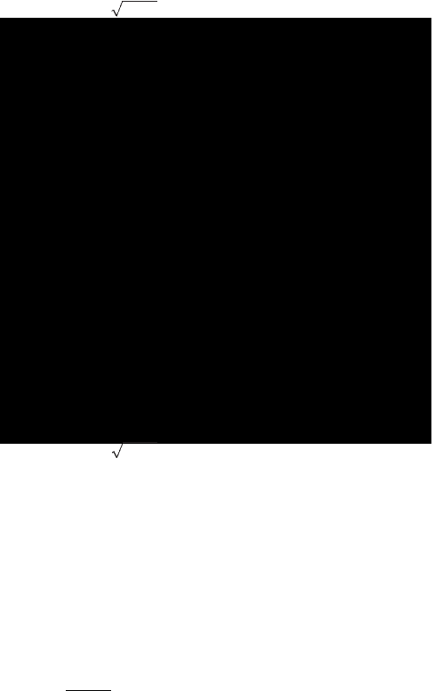
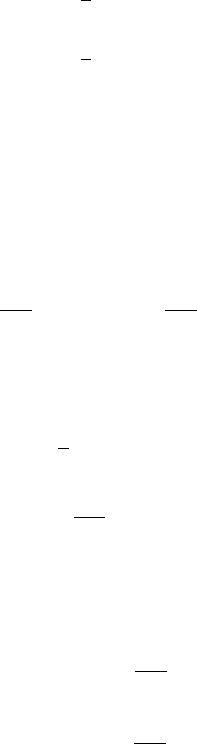
Figure 1.1 A Kruskal–Szekeres diagram. [After Shapiro and Teukolsky (1983).]
clearly blows up at the origin, showing that the tidal gravitational field becomes infinite at
the center of the black hole.
One alternative coordinate choice that removes the coordinate singularity at r = 2M is
the Kruskal–Szekeres coordinate system.
11
In these coordinates, the metric (1.51) takes
the form
ds
2
=
32M
3
r
e
−r/2M
−dv
2
+ du
2
+r
2
dθ
2
+r
2
sin
2
θdφ
2
. (1.55)
The original Schwarzschild coordinate system covers only half of the spacetime man-
ifold, while Kruskal–Szekeres coordinates cover the entire manifold. This situation is
revealed in the Kruskal–Szekeres diagram shown in Figure 1.1. In this spacetime diagram
the timelike coordinate v is plotted vertically and the spacelike coordinate u is plotted
horizontally. Region I corresponds to the original region r > 2M, “our Universe”. Region
II is the region r < 2M, the “black hole interior”. Regions III and IV represent the “other
Universe”: region III has r > 2M and is asymptotically flat, while region IV has r < 2M
and can describe a “white hole”. The relationship between Kruskal–Szekeres coordinates
u and v and Schwarzschild coordinates t and r depends on the quadrant in the u–v plane.
11
Kruskal (1960); Szekeres (1960).
12 Chapter 1 General relativity preliminaries
We h ave
u =±
(
r/2M − 1
)
1/2
e
r/4M
cosh(t/4M)
v =±
(
r/2M − 1
)
1/2
e
r/4M
sinh(t/4M)
r ≥ 2M, (1.56)
where the upper sign refers to region I and the lower to region III, while
u =±
(
r/2M − 1
)
1/2
e
r/4M
sinh(t/4M)
v =±
(
r/2M − 1
)
1/2
e
r/4M
cosh(t/4M)
r ≤ 2M, (1.57)
where the upper sign refers to region II, and the lower sign to region IV. The inverse
transformations are
(r/2M − 1)e
r/2M
= u
2
− v
2
in I, II, III, IV ; (1.58)
and
t =
4M tanh
−1
(v/u) in regions I and III,
4M tanh
−1
(u/v) in regions II and IV.
(1.59)
In the Kruskal–Szekeres diagram, curves of constant r are hyperbolae with asymptotes u =
±v, while curves of constant t are straight lines through the origin.
12
From equation (1.58)
we see that the singularity at r = 0isatv =±(1 + u
2
)
1/2
and is shown in Figure 1.1 as
a saw-toothed curve. Note that radial light rays propagate along 45
◦
lines in the Kruskal–
Szekeres diagram. Thus timelike worldlines propagating in region II cannot escape the
black hole interior and must hit the singularity at r = 0.
Other forms of the Schwarzschild metric are useful, particularly in numerical computa-
tions. For example, the Schwarzschild metric in isotropic radial coordinates is
ds
2
=−
1 − M/2
¯
r
1 + M/2
¯
r
2
dt
2
+
1 +
M
2
¯
r
4
d
¯
r
2
+
¯
r
2
dθ
2
+ sin
2
θdφ
2
, (1.60)
where the transformation between areal and isotropic coordinates is
r =
¯
r
(
1 + M/2
¯
r
)
2
. (1.61)
The inverse transformation is
¯
r =
1
2
r − M ±
(
(r − 2M)
)
1/2
, (1.62)
and is double valued. Note that the isotropic coordinate
¯
r describes only the region of
Schwarzschild geometry with r ≥ 2M. The black hole event horizon is located at
¯
r = M/2
in these coordinates. We will have occasion to use this and other coordinate systems for
analyzing Schwarzschild black holes in later chapters.
12
See also Figure 8.1 for a more detailed plot of region I; there r
s
denotes areal radius.

1.2 Black holes 13
Kerr black holes
The solution to Einstein’s equations describing a stationary, rotating, uncharged black hole
of mass M and angular momentum J in vacuum may be expressed in Boyer–Lindquist
coordinates
13
in the form
ds
2
=−
1 −
2Mr
dt
2
−
4aMrsin
2
θ
dtdφ +
dr
2
+ dθ
2
+
r
2
+ a
2
+
2a
2
Mrsin
2
θ
sin
2
θdφ
2
, (1.63)
where
a ≡ J/M,≡ r
2
− 2Mr + a
2
,≡ r
2
+ a
2
cos
2
θ, (1.64)
and where the black hole is rotating in the +φ direction. Note that when the angular
momentum parameter a is zero, the solution reduces to the Schwarzschild metric (1.51).
The spin is restricted to the range 0 ≤ a/M ≤ 1. The rotating black is stationary and
axisymmetric, hence the spacetime possesses two Killing vectors ∂
t
and ∂
φ
. Thus, test
particles moving in the field of a rotating black hole conserve their energy E =−p
t
and
axial component of angular momentum l = p
φ
.
14
Circular orbit parameters for particles
moving in the equatorial plane of a rotating black hole are analytic and discussed in many
references.
15
The horizon of the black hole is located at r
+
, the largest root of the equation = 0,
r
+
= M +
M
2
− a
2
1/2
. (1.65)
The static limit is the surface within which no static observers exist; it resides at r
0
,the
largest root of g
tt
= 0:
r
0
= M +
M
2
− a
2
cos
2
θ
1/2
. (1.66)
The region between the horizon and static limit is called the ergosphere; in this region all
timelike observers are dragged around the hole with angular velocity >0.
Global theorems
A number of extraordinary theorems have been proven over the years that address very
general, global properties of black hole spacetimes. We defer to other textbooks for detailed
derivation and discussion of these elegant results.
16
Some of these results are encapsulated
13
Boyer and Lindquist (1967).
14
There is an additional constant of the motion, called Carter’s “fourth constant” that is related to total angular momentum;
Carter (1968).
15
Bardeen et al. (1972); Shapiro and Teukolsky (1983).
16
Hawking and Ellis (1973); Misner et al. (1973); Wald (1984); Poisson (2004), and references therein.
14 Chapter 1 General relativity preliminaries
in the “four laws of black hole mechanics”, which are remarkably similar to the laws of
thermodynamics and demonstrate that black holes act like thermodynamic systems. As
an example, consider the second law of black hole dynamics, proven by Hawking:
17
In
an isolated system, the sum of the surface areas of all black holes can never decrease.
Consider the implication of this area theorem for a Kerr black hole. The surface area is the
area
A of the horizon at some instant of time. Setting r = r
+
and t = constant and using
equation (1.63) gives the 2-metric on the horizon,
(2)
ds
2
=
r
2
+
+ a
2
cos
2
θ
dθ
2
+
(2Mr
+
)
2
r
2
+
+ a
2
cos
2
θ
sin
2
θdφ
2
, (1.67)
from which we may derive
A according to
A =
(2)
gdθdφ, (1.68)
where g is the determinant of the 2-metric. Evaluating equation (1.68) yields
A = 8π M
M + (M
2
− a
2
)
1/2
, (1.69)
which reduces to
A = 4π(2M)
2
when a = 0. If we define an irreducible mass M
irr
accord-
ing to
A ≡ 16π M
2
irr
, (1.70)
then we may write (1.69)as
M
2
= M
2
irr
+
J
2
4M
2
irr
. (1.71)
Equation (1.71) states that the mass of a Kerr black hole is composed of an irreducible
contribution plus a rotational kinetic energy contribution.
18
According to the area theorem,
only the rotational energy contribution can be tapped as a source of energy by an external
system interacting with the hole, since the irreducible mass can never decrease. For a
system of black holes, the sum of the squares of the irreducible masses of all black holes
can never decrease, at least classically.
Taking quantum mechanics into account, a black hole is characterized by a well-defined
temperature T , emits thermal Hawking radiation, and has an entropy S proportional to its
area according to
S =
kc
3
G
¯
h
A
4
, (1.72)
where k is Boltzmann’s constant,
¯
h is Planck’s constant, and where we have temporarily
restored G and c.
19
When black hole evaporation via Hawking radiation is taken into
17
Hawking (1971, 1972, 1973).
18
Christodoulou (1970); Christodoulou and Ruffini (1971).
19
Bekenstein (1973, 1975); Hawking (1974, 1975).

1.3 Oppenheimer–Volkoff spherical equilibrium stars 15
account, the generalized second law of black hole thermodynamics states that the total
entropy, the sum of black hole and radiation entropies, never decreases.
20
1.3 Oppenheimer–Volkoff spherical equilibrium stars
The metric describing the gravitational field of a spherical star may be written in the form
ds
2
=−e
2
dt
2
+ e
2λ
dr
2
+r
2
d
2
, (1.73)
where and λ are functions of t and r in general, but functions of areal radius r alone in
the case of static equilibrium, and d
2
= dθ
2
+ sin
2
θdφ
2
. Suppose that the stellar matter
can be described as a perfect fluid and that the equation of state can be written in the form
ρ = ρ(n
b
, s), where ρ is the total mass-energy density, n
b
is the baryon density and s is
the specific entropy. The first law of thermodynamics then yields the pressure,
P = n
2
b
∂(ρ/n
b
)
∂n
b
= P(n
b
, s). (1.74)
In many applications the equation of state reduces to a one-parameter equation of state
of the form
P = P(ρ). (1.75)
Such is the case, for example, when the matter is isentropic, as in the case of cold nuclear
matter (s = 0) or matter in a supermassive star (s = constant).
The equations of stellar structure for spherical equilibrium stars in general relativity are
coupled, first-order, ordinary differential equations. Defining a new metric function m(r)
by
e
λ
≡
1 −
2m
r
−1
, (1.76)
Einstein’s equations give
dm
dr
= 4πr
2
ρ, (1.77)
dP
dr
=−
ρm
r
2
1 +
P
ρ
1 +
4π Pr
3
m
1 −
2m
r
−1
, (1.78)
d
dr
=−
1
ρ
dP
dr
1 +
P
ρ
−1
. (1.79)
20
Our treatment throughout focuses on classical general relativity, since it provides an excellent description for the
astrophysical systems that we shall consider. Only for “mini” black holes of mass M
<
∼
10
15
g is the evaporation time
scale shorter than the age of the Universe.

16 Chapter 1 General relativity preliminaries
The above set of equations is sometimes called the Oppenheimer–Volkoff or OV equa-
tions, and sometimes the Tolman–Oppenheimer–Volkoff or TOV equations, of spherical
equilibrium.
21
The Newtonian limit is recovered by choosing P ρ and m r.
The quantity m(r) can be interpreted as the “mass interior to radius r”. The total mass
of the star is given by equation (1.77),
M =
R
0
4πr
2
ρdr, (1.80)
where R is the stellar radius (the point where P = ρ = 0). Note that the quantity m(R)
must equal M so that the interior metric coefficient (1.76) will match smoothly onto the
exterior vacuum Schwarzschild metric (1.51). The total rest-mass M
0
is determined from
M
0
=
R
0
4πr
2
ρ
0
(1 − 2m/r)
−1/2
dr, (1.81)
where ρ
0
is the rest-mass density. The quantities ρ and ρ
0
are related by
ρ = ρ
0
(
1 +
)
, (1.82)
where is the internal energy density per unit rest mass. For baryonic matter, ρ
0
= n
b
m
b
,
where m
b
is the mean baryonic rest mass. For bound configurations we have M < M
0
:
the total mass-energy M includes negative gravitational potential energy in addition to the
rest-mass-energy M
0
and internal energy.
Equations (1.77)–(1.79) are straightforward to integrate numerically to construct a stellar
model: First choose a central density, ρ
c
, for which the equation of state (1.75)givesthe
central pressure P
c
. The central boundary conditions
m = 0andP = P
c
at r = 0, (1.83)
allow one to integrate equations (1.77) and (1.78) beginning at the origin, to get m(r)
and P(r), hence ρ(r), for all 0 ≤ r ≤ R.Itisusefultointegrateequation(1.79) simul-
taneously with the other two equations, choosing an arbitrary value for (r = 0). Since
equation (1.79) is linear in , one can then add a constant value to everywhere so that
it matches smoothly onto the Schwarzschild solution at the surface:
(R) =
1
2
ln
1 −
2M
R
. (1.84)
Integrating the OV equations analytically for a uniform density, incompressible star
shows that equilibrium is possible only if
2M
R
<
8
9
. (1.85)
In fact, the above limit for the maximum “compaction” M/R of a uniform density sphere
applies to spheres of arbitrary density profile, provided the density does not increase
outwards.
22
21
Oppenheimer and Volkoff (1939); Tolman (1939).
22
See, e.g., Weinberg (1972), Section 11.6. Note that this limit is sometimes referred to as the “Buchdahl limit”; Buchdahl
(1959).
1.3 Oppenheimer–Volkoff spherical equilibrium stars 17
Polytropes
Some of the simplest and most useful families of equilibrium models are constructed from
an isentropic equation of state of the form,
P = Kρ
0
(K ,constants), (1.86)
where ρ
0
is the rest-mass density. The constant K is the polytropic gas constant and
the quantity n defined by ≡ 1 + 1/n is called the polytropic index. Stellar models
constructed from such an equation of state are called polytropes. For an equation of
stategivebyequation(1.86), we find from the first law of thermodynamics (or from
equation 1.74) that ρ
0
= P/( − 1) and ρ = ρ
0
+ P/( − 1).
There are a number of physically interesting stars that can be modeled as polytropes
in a first approximation. For example, stars supported against collapse by the pressure
of noninteracting, nonrelativistic, degenerate fermions can be modeled as n = 3/2 poly-
tropes, while stars supported by noninteracting, ultrarelativistic, degenerate fermions can
be modeled as n = 3 polytropes. In such cases, lower-mass objects are constructed from
nonrelativistic fermions, while higher-mass objects are constructed from highly relativistic
fermions. White dwarfs, which are supported by the pressure of degenerate electrons, and
neutron stars, which are supported by degenerate neutrons, are members of this class of
models.
23
When nuclear interactions are included, high-mass neutron stars are better rep-
resented by a “stiffer” equation of state, but the resulting models are often crudely modeled
as n = 1 relativistic polytropes. Another example is a star supported by thermal radiation
pressure at constant specific entropy, which can be modeled as an n = 3 polytrope.
24
When using a polytropic equation of state to construct stellar equilibrium models, it is
always possible to scale out the constant K . In gravitational units K
n/2
has units of length,
so that we can introduce a new set of nondimensional quantities, often denoted by a bar:
¯
r ≡ K
−n/2
r, ¯ρ
0
≡ K
n
ρ
0
, ¯ρ ≡ K
n
ρ,
¯
P ≡ K
n
P,
¯
M ≡ K
−n/2
M,
¯
M
0
≡ K
−n/2
M
0
. (1.87)
One can thus set K = 1 in numerical integrations and either use the above relations to scale
the results to more physical values of K , or express answers in terms of nondimensional
ratios that are independent of K (e.g., R/M, M
2
ρ
0
,etc.).
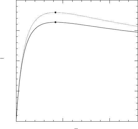
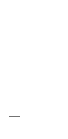
In Figure 1.2 we plot the equilibrium sequence for n = 1 polytropes as an example. The
turning point along a curve of equilibrium mass vs. central density, like the ones plotted
here, identifies the maximum mass configuration. It also marks the onset of radial dynam-
ical instability along the sequence. In particular, configurations to the left of the turning
point, where dM/dρ
c
> 0, are dynamically stable to small radial perturbations and will
23
For ultrarelativistic degenerate fermions there is a maximum mass limit, which for a white dwarf is called the
Chandrasekhar limit and is about 1.4M
. S. Chandrasekhar received the Nobel prize in 1983, in part for identifying
this important limit (Chandrasekhar 1931).
24
For a thorough discussion of polytropes and more detailed models of compact objects like white dwarfs, neutron stars
and supermassive stars and their stability properties, see Shapiro and Teukolsky (1983) and references therein.
18 Chapter 1 General relativity preliminaries
0
0
0.05
0.1
0.15
0.2
0.5 1
M
r
c
Figure 1.2 Equilibrium sequence for n = 1 spherical polytropes. The total mass-energy
¯
M (solid line) and the
rest-mass
¯
M
0
(dotted line) are plotted as functions of the central mass-energy density ¯ρ
c
along the sequence. The
dots indicate the turning points, or the location of the maximum mass configuration, on each curve. The turning
points occur at the same density along the two curves.
undergo small amplitude radial oscillations when subjected to such perturbations, while
configurations to the right, where dM/dρ
c
< 0, are unstable and can undergo catastrophic
collapse. For the case of an n = 1 polytrope, the turning point occurs at ¯ρ
c
= 0.420 where
¯
M = 0.164 and
¯
M
0
= 0.180.
25
1.4 Oppenheimer–Snyder spherical dust collapse
Among the most useful analytical solutions of the Einstein equations is the solution of
Oppenheimer and Snyder (1939) describing the collapse of a spherical star with uniform
density and zero pressure to a Schwarzschild black hole. Though it treats a highly idealized
collapse scenario, the analysis is exact and fully nonlinear. The Oppenheimer–Snyder, or
OS, solution illustrates many generic features of gravitational collapse and black hole
formation. Since the solution is analytic, it is simple to work with and is often used to test
and calibrate numerical codes designed to deal with more complicated cases, as we shall
see later. Because of the important role that it plays in numerical relativity, we present this
classic solution here.
25
We recommend that students newly aquainted with computational physics integrate the OV equations numerically for
an n = 1 polytrope and reproduce Figure 1.2, together with the quoted values at the turning points, before moving on
to some of the more difficult computational challenges that lie ahead.
1.4 Oppenheimer–Snyder spherical dust collapse 19
In the OS solution, each fluid element in the star of mass M follows a radial geodesic,
as there is no pressure. The interior metric is given by the familiar (closed Friedmann) line
element
ds
2
=−dτ
2
+ a
2
(dχ
2
+ sin
2
χ d
2
). (1.88)
Here τ is the time coordinate, measured from the onset of collapse, χ is a Lagrangian or
comoving radial coordinate and a is related to τ implicitly through the conformal time
parameter η,
a =
1
2
a
m
(1 + cos η), (1.89)
τ =
1
2
a
m
(η + sin η). (1.90)
The parameter η varies between 0 and π. The spatial coordinates of a fluid element are
comoving, with χ, θ and φ remaining fixed during the collapse, and the time coordinate
τ measures the proper time of a fluid element. This choice of coordinates is called syn-
chronous, Gaussian normal or geodesic. The surface of the star is located at some fixed
radial coordinate χ = χ
0
.
The exterior metric is given by the Schwarzschild line element,
ds
2
=−
1 −
2M
r
s
dt
2
+
1 −
2M
r
s
−1
dr
2
s
+r
2
s
d
2
. (1.91)
The surface of the star in these coordinates is at r
s
= R(τ ) and follows a radial geodesic
according to
R =
1
2
R
0
(1 + cos η), (1.92)
τ =
R
3
0
8M
1/2
(η + sin η), (1.93)
where the subscript ‘0’ denotes the value of the radius at t = 0. Matching the interior and
exterior solutions at the surface yields
a
m
=
R
3
0
2M
1/2
, (1.94)
sin χ
0
=
2M
R
0
1/2
. (1.95)
According to the above equation, χ
0
must lie in the range 0 ≤ χ
0
≤ π/2.
The fluid 4-velocity u
a
= ∂
τ
satisfies the geodesic equations (1.27). In these coordinates,
the rest-mass density ρ
0
(which equals the total mass-energy density ρ, since, in the absence
20 Chapter 1 General relativity preliminaries
0
0
5
10
15
20
25
12
0.1 0.25 0.5 1.0
r
s
/M
τ/M
3456
Figure 1.3 Spacetime diagram for Oppenheimer–Snyder spherical collapse to a Schwarzschild black hole. The
initial stellar (areal) radius is R/M = 5. Worldlines of spherical fluid shells are shown as solid lines and labeled
by the interior mass fraction. The event horizon is indicated by the dotted line. The shaded area denotes the
region of trapped surfaces and its outer boundary is the apparent horizon.The inner boundary of the region of
trapped surfaces is denoted by the dashed line. The spacetime singularity that forms at the center is indicated by
the zig-zag line.
of pressure, there is no internal energy either) is a function of proper time alone,
ρ
0
(τ )
ρ
0
(0)
= Q
−3
(τ ), (1.96)
where
Q(τ ) =
a
a
m
=
1
2
(1 + cos η). (1.97)
In our synchronous coordinate system the star thus remains homogeneous throughout the
collapse. The proper time for the star to undergo complete collapse is τ
coll
= π (R
3
0
/8M)
1/2
,
as is evident from equations (1.92) and (1.93). At this time a central singularity forms at
the center of the star.
It is both instructive and straightforward to probe the spacetime geometry of OS collapse.
The spacetime diagram in Figure 1.3 shows the worldlines of infalling Lagrangian fluid
elements as well as the location of the black hole event horizon. The event horizon
first forms at the center and grows monotonically outward to encompass the entire star.
Determining the event horizon requires that the global spacetime be known. Since it is
known analytically in this example, the location of the event horizon can be determined
quite easily: Outgoing null rays in the interior satisfy ds
2
= 0ordτ = a(τ )dχ from
equation (1.88). Using equations (1.89) and (1.90) this yields dχ/dη = 1. Thus an outgoing
ray emitted at η = η
e
, χ = χ
e
follows the trajectory
χ = χ
e
+ (η − η
e
). (1.98)
The event horizon is the trajectory of an outgoing null ray that originates at the stellar
center and intersets the surface of the star just when the surface crosses R = 2M. This
trajectory traces the worldline of the the last ray that manages to escape to infinity from