Baumgarte T., Shapiro S. Numerical Relativity. Solving Einstein’s Equations on the Computer

Подождите немного. Документ загружается.

3.1 Conformal transformations 61

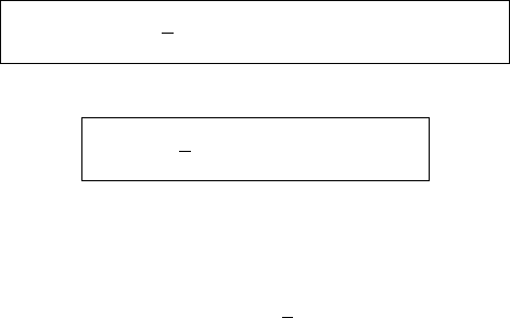
Figure 3.2 Schematic embedding diagram of the geometry described by metric (3.23) for two black holes at a

moment of time symmetry. This is the three-sheeted topology, which does not satisfy an isometry across each

throat.

we obtain the solution simply by adding the individual contribution of each black hole

according to

ψ = 1 +



. (3.23)

Here r

=|x

− C

| is the (coordinate) separation from the center C

of the αth black

hole. The total mass of the spacetime is the sum of the coefﬁcients

. However, since

the total mass will also include contributions from the black hole interactions,

can

be identiﬁed with the mass of the αth black hole only in the limit of large separations.

Particularly interesting astrophysically and for the generation of gravitational waves is the

case of binary black holes, in which case (3.23) reduces to

ψ = 1 +

. (3.24)

This simple solution to the constraint equations for two black holes instantaneously at rest

at a moment of time symmetry can be used as initial data for head-on collisions of black

holes (see Chapter 13.2).

We can now deﬁne mappings equivalent to (3.20), which represent reﬂections through

the αth throat. In general, the existence of other black holes destroys the symmetry that we

found for a single black hole. Each Einstein–Rosen bridge therefore connects to its own

asymptotically ﬂat Universe. Drawing an embedding diagram for such a geometry yields

several different “sheets”, where each sheet corresponds to one Universe. A geometry

containing N black holes may contain up to N + 1 different asymptotically ﬂat universes

(see Figure 3.2).

If desired, however, the isometry across the throats can be restored as follows. Recall

that equation (3.16) is equivalent to the Laplace equation in electrostatics, so that we

62 Chapter 3 Constructing initial data

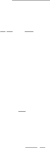
Figure 3.3 Schematic embedding diagram of a “symmetrized” two black hole solution. This is a two-sheeted

topology, in which two Einstein–Rosen bridges connect two identical, asymptotically ﬂat universes.

Figure 3.4 Illustration of a wormhole black hole solution.

can borrow the method of spherical inversion images

to analyze it. For each throat

in (3.23) we can add terms inside that throat that correspond to images of the other

black holes. Doing so, the solution (3.23) becomes “symmetrized” so that the reﬂection

through each throat is again an isometry. In other words, each Einstein–Rosen bridge

connects to the same asymptotically ﬂat Universe, and the geometry consists of only two

asymptotically ﬂat universes, which are connected by several Einstein–Rosen bridges (see

Figure 3.3).

For two equal-mass black holes we may also interpret this solution as a wormhole black

hole solution. To see this, consider the solution illustrated in Figure 3.3 for two throats of

equal mass. Cut off the bottom Universe at the two throats, which leaves two “open-ended”

throats hanging down from the top Universe. We can now identify these two open ends

with each other, effectively gluing them together. As illustrated in Figure 3.4, the two

throats now form a “wormhole” that connects to a single, asymptotically ﬂat (but multiply

connected) Universe. Given the original isometry conditions across the throats, and given

See Misner (1963); Lindquist (1963).

3.1 Conformal transformations 63

that they have the same mass, the resulting metric is smooth across the throat and a valid

solution to the Hamiltonian constraint.

In cylindrical coordinates the metric becomes

= ψ

(dρ

+ dz

+ ρ

dφ

), (3.25)

where the corresponding conformal factor is given by

ψ = 1 +

∞



n=1

sinh(nµ)





+ (z + z

)



+ (z − z

)



. (3.26)

Here z

= coth(nµ), and µ is a free parameter. In exercise 3.21 we will see that the total

mass of this system, which we will identify with the “ADM mass” in Section 3.5,is

ADM

= 4

∞



n=1

sinh(nµ)

. (3.27)

The proper distance L along the spacelike geodesic connecting the throats, or equivalently

the proper length of a geodesic loop through the wormhole, is

L = 2



1 + 2µ

∞



n=1

sinh(nµ)



. (3.28)

The parameter µ is seen to parametrize both the mass and separation of the two holes.

Since the solution can be rescaled to arbitrary physical mass, µ effectively determines

the dimensionless ratio L/M

ADM

, the parameter that, apart from mass, distinguishes one

binary from another in this class of initial data.

As we have seen, the solution to the Hamiltonian constraint equation for a system

containing more than one vacuum black hole at a moment of time symmetry is by no

means unique. The different solutions satisfy different inversion properties on the throats,

and represent solutions to the Hamiltonian constraint in different topologies.Ifviewed

from only one “Universe”, the different solutions satisfy different boundary conditions on

the throats. This difference leads to a different initial gravitational wave content in the

sense that the dynamical evolution of these initial data would lead to different gravitational

wave signals, at least for the initial burst. We will discuss initial data for multiple black

holes in much more detail in Chapter 12, and will postpone a further discussion of these

issues until then.

Exercise 3.5 Brill waves are deﬁned as nonlinear, axisymmetric gravitational waves

in vacuum spacetimes that admit a moment of time symmetry.

Consider a spatial

metric in cylindrical coordinates

= ψ



(dρ

+ dz

) + ρ

dφ



, (3.29)

Misner (1960) originally derived this solution by starting with a 3-dimensional “donut” solution. Part of this donut

ultimately forms the tube of the wormhole, while one point on the original donut is pulled apart towards inﬁnity to

form the asymptotically ﬂat Universe.

See, e.g., Anninos et al. (1994).

Brill (1959). See also Eppley (1977).

64 Chapter 3 Constructing initial data

where q(ρ,z) is an arbitrary, axisymmetric function that introduces a deviation

from conformal ﬂatness and that can be considered a measure of the gravitational

wave amplitude. Show that at a moment of time symmetry the conformal factor ψ

satisﬁes

∇

ψ =−



∂

∂ρ

∂

∂z



, (3.30)

where ∇

is the ﬂat space Laplace operator in three dimensions. Solving this non-

linear elliptic equation provides a surprisingly simple way of constructing nonlinear

gravitational wave initial data.

3.1.3 Conformal transformation of the extrinsic curvature

Return now to the development of the conformal decomposition of the constraint equations.

We have conformally transformed the spatial metric, but before we proceed we also have

to decompose the extrinsic curvature. It is convenient to split K

into its trace K and a

traceless part A

according to

= A

K, (3.31)

and to conformally transform K and A

separately. A priori it is not clear how to trans-

form K and A

, and our only guidance for inventing rules is that the transformation

should bring the constraint equations into a simple and solvable form. Consider the

transformations

= ψ

(3.32)

K = ψ

K , (3.33)

where α and β are two so far undetermined exponents.

Exercise 3.6 Show that the divergence of any symmetric, traceless tensor A

which

transforms according to (3.32) satisﬁes

= ψ

−10

(ψ

10+α

). (3.34)

Exercise 3.6 immediately suggests the choice α =−10, i.e.,

= ψ

−10

, (3.35)

which implies A

= ψ

−2

. With this choice a symmetric traceless tensor A

has zero

divergence if and only if

does. This is not the only possible choice for the exponent α,

though, and we will use a different scaling in Chapter 11.

Inserting the above expressions into the momentum constraint (3.2) yields

−10

−

β−4

¯γ

K −

βψ

β−5

K ¯γ

ψ = 8π S

. (3.36)

3.1 Conformal transformations 65

Our desire to simplify equations motivates the choice β = 0, so that we treat K as a

conformal invariant, K =

K . With these choices, the Hamiltonian constraint now becomes

ψ − ψ

R −

+ ψ

−7

=−16πψ

ρ, (3.37)

and the momentum constraint is

−

¯γ

K = 8πψ

. (3.38)

Exercise 3.7 Consider the weak-ﬁeld limit of equation (3.37) under the same

assumptions as in Exercise 2.28. Then compare with the Poisson equation for the

Newtonian gravitational potential  to show that

ψ = 1 −

 (3.39)

in the weak-ﬁeld limit, assuming suitable boundary conditions for ψ and .

In addition to the spatial metric and extrinsic curvature, it may also be necessary

to transform the matter sources ρ and S

in (3.37) and (3.38) to insure uniqueness of

solutions.

We will largely ignore this issue in this chapter, but it is nevertheless instructive

to discuss its origin in passing.

We start by considering the linear equation

∇

u = fu (3.40)

on some domain .Here f is some given function, and we will assume u = 0onthe

boundary ∂.If f is nonnegative everywhere, we can apply the maximum principle to

show that u = 0 everywhere. The point is that if u were nonzero somewhere in ,say

positive, then it must have a maximum somewhere. At the maximum the left hand side

of (3.40) must be negative, but the right hand side is nonnegative if f ≥ 0, which is

a contradiction. Clearly, the argument works the same way if u is negative somewhere,

implying that u = 0everywhereif f ≥ 0.

Now consider the nonlinear equation

∇

u = fu

, (3.41)

and assume there exist two positive solutions u

and u

≥ u

that are identical, u

= u

on the boundary ∂. The difference u = u

− u

must then satisfy an equation

∇

u = nf

n−1

u, (3.42)

where

u is some positive function satisfying u

≤

u ≤ u

. Applying the above argument to

u, we see that the maximum principle implies u = 0 and hence uniqueness of solutions

See, e.g., Yo r k , J r . (1979).

66 Chapter 3 Constructing initial data

if and only if nf ≥ 0, i.e., if the coefﬁcient and exponent in the source term of (3.41)have

thesamesign.

Inspecting the Hamiltonian constraint (3.37) we see that the matter term −16πψ

features the “wrong signs”: it has a negative coefﬁcient (assuming a positive matter density

ρ), but a positive exponent for ψ. Therefore the maximum principle cannot be applied,

and the uniqueness of solutions cannot be established. Exercise 3.8 explores this issue for

an analytical example.

Exercise 3.8 Consider the Hamiltonian constraint (3.37) at a moment of time

symmetry, K

= 0, and under the assumption of conformal ﬂatness and spherical

symmetry. Also assume boundary conditions ∂

ψ = 0atr = 0, and ψ → 1for

r →∞. Now consider a constant density star with

ρ(r) =



, r < r

0, r ≥ r

(3.43)

In the following we will consider r

as given, and will study the solutions as a

function of the density ρ

(a) Show that the Sobolev functions

(r) ≡

(νr

)

1/2



+ (νr

)



1/2

(3.44)

satisfy the equation

∂

∂r



∂u

∂r



=−3u

(3.45)

for any constant ν. Conclude that for r < r

the solution for ψ is given by ψ

int

= Cu

and ﬁnd the value of C.

(b) For r ≥ r

the solution is given by ψ

= 1 + µ/r,whereµ is another yet

undetermined constant. The interior and exterior solutions already satisfy the differ-

ential equation and boundary conditions individually, but to obtain a global solution

we still need to enforce that their function values and ﬁrst derivatives match at r = r

These two conditions ﬁx the constants µ and ν for a given background density ρ

Show that the conditions can be combined to yield an equation for ν,

2π

(ν), (3.46)

where f (ν) ≡ ν

/(1 + ν

)

>ρ

crit

2πr

. (3.47)

Further show that for any ρ

<ρ

crit

,therearetwo solutions ν, and hence two distinct

solutions ψ, that satisfy the Hamiltonian constraint for the matter distribution (3.43).

Clearly, the solutions are not unique.

See Baumgarte et al. (2007) for a further exploration of this solution as well as related issues. Note that for homogeneous

ﬂuid stars in hydrostatic equilibrium, there is only one physically relevant solution to the Hamiltonian constraint

3.2 Conformal transverse-traceless decomposition 67

Uniqueness of solutions can be restored, however, by introducing a conformal rescaling

of the density. With ρ = ψ

¯ρ,whereδ ≤−5andwhere ¯ρ is now considered a given

function, the matter term carries the “right signs”, and the maximum principle can be

applied to establish the uniqueness of solutions. Furthermore, in the example of exercise

3.8 the solutions are unique locally even for unscaled density sources – at least for matter

densities smaller than the critical density – and there is some evidence that this property is

generic.

If so, a numerical algorithm can still iterate towards the desired solution, given

suitable background data, as long as the iteration starts with a sufﬁciently “close” initial

guess.

Most decompositions use the conformal rescaling of the spatial metric and the extrinsic

curvature as introduced above. Different decompositions then proceed by decomposing

in different ways. In the following sections we will discuss the transverse-traceless and

the conformal thin-sandwich decompositions.

3.2 Conformal transverse-traceless decomposition

Any symmetric, traceless tensor can be split into a transverse-traceless part that is diver-

genceless and a longitudinal part that can be written as a symmetric, traceless gradient of

a vector. We can therefore decompose

, (3.48)

where the transverse part is divergenceless,

= 0, (3.49)

and where the longitudinal part satisﬁes

−

¯γ

≡ (

LW)

. (3.50)

Here W

is a vector potential, and it is easy to see that the longitudinal operator or vector

gradient

L produces a symmetric, traceless tensor.

We can now write the divergence of

(

LW)

(

) +

≡ (



W )

, (3.51)

where



is the vector Laplacian.

equation. Moreover, the critical density at which the central pressure becomes inﬁnite in an equilibrium star, which

occurs when M/R = 4/9, is smaller than the critical density given by equation (3.47). Hence the latter density is never

reached along an equilibrium sequence of stars of constant mass M but increasing density and compaction.

See Baumgarte et al. (2007); Walsh (2007).

Vectors ξ

satisfying (

Lξ )

= 0 are called conformal Killing vectors (see exercise A.7 in Appendix A), which suggests

why

L is also called the conformal Killing operator.

68 Chapter 3 Constructing initial data

Exercise 3.9 Consider a ﬂat conformally related metric ¯γ

= η

in spherical polar

coordinates, and assume that the only nonvanishing component of the vector W

the radial component W

. Then show that the only nonzero component of the vector

Laplacian is

(



W )

∂

∂r



∂

∂r







. (3.52)

Note that

and

are transverse and longitudinal with respect to the conformal

metric ¯γ

, which is why this decomposition is called the conformal transverse-traceless

decomposition. Alternatively, one can adopt a physical transverse-traceless decomposition,

where the corresponding tensors are transverse and longitudinal with respect to the physical

metric γ

Inserting the conformally related quantities into the momentum constraint (3.38) yields

(



W )

−

¯γ

K = 8πψ

. (3.53)

The Hamiltonian constraint remains in its form (3.37). We now see that we can freely

choose the conformally related metric ¯γ

, the mean curvature K and the transverse-

traceless part of the conformally related extrinsic curvature,

. Given these choices,

we can then solve the Hamiltonian constraint (3.37) for the conformal factor ψ and the

momentum constraint (3.53) for the vector potential W

. Knowing these quantities, we

can construct ﬁnally the physical solutions γ

and K

. We summarize this conformal

transverse-traceless, or “CTT”, decomposition in Box 3.1.

Box 3.1 The conformal transverse-traceless (CTT) decomposition

Freely speciﬁable variables are ¯γ

, K and

. Given these, the momentum constraint

(



W )

−

¯γ

K = 8πψ

(3.54)

is solved for W

, and the Hamiltonian constraint

ψ − ψ

R −

+ ψ

−7

=−16πψ

ρ, (3.55)

where

+ (

LW)

, (3.56)

is solved for ψ. The physical solution is then constructed from

= ψ

¯γ

(3.57)

and

= A

K = ψ

−2

K. (3.58)

3.2 Conformal transverse-traceless decomposition 69

Before discussing some simple solutions to equation (3.53), it is useful to count degrees

of freedom again, as we did at the beginning of this chapter. We started out with six

independent variables in both the spatial metric γ

and the extrinsic curvature K

. Split-

ting off the conformal factor ψ left ﬁve degrees of freedom in the conformally related

metric ¯γ

(once we have speciﬁed its determinant ¯γ ). Of the six independent variables

in K

we moved one into its trace K , two into

(which is symmetric, traceless, and

divergenceless), and three into

(which is reﬂected in its representation by a vector). Of

the 12 original degrees of freedom, the constraint equations determine only four, namely

the conformal factor ψ (Hamiltonian constraint) and the longitudinal part of the traceless

extrinsic curvature

(momentum constraint). Four of the remaining eight degrees of

freedom are associated with the coordinate freedom – three spatial coordinates hidden in

the spatial metric and a time coordinate that is associated with K . This leaves four physical

degrees of freedom undetermined – two in the conformally related metric ¯γ

, and two

in the transverse part of the traceless extrinsic curvature

. These freely speciﬁable

degrees of freedom carry the dynamical degrees of freedom of the gravitational ﬁelds. All

others are either ﬁxed by the constraint equations or represent coordinate freedom.

We have reduced the Hamiltonian and momentum constraints to equations for the

conformal factor ψ and the vector potential W

, from which the longitudinal part of the

extrinsic curvature is constructed. These quantities can be solved for only after choices

have been made for the remaining quantities in the equations, namely the conformally

related metric ¯γ

, the transverse-traceless part of the extrinsic curvature

, the trace

of the extrinsic curvature K , and, if present, any matter sources. The choice of these

background data has to be made in accordance with the physical or astrophysical situation

that one wants to represent. Physically, the choice affects the gravitational wave content

present in the initial data, in the sense that a dynamical evolution of data constructed with

different background data leads to different amounts of emitted gravitational radiation. It

is often not clear how a suitable background can be constructed precisely, and we will

return to this issue on several occasions. Given its loose association with the transverse

parts of the gravitational ﬁelds, one often sets

equal to zero in an attempt to minimize

the gravitational wave content in the initial data.

The freedom in choosing the background data can also be used to simplify the equations.

Focus again on vacuum solutions, so that ρ = S

= 0. We will now assume maximal slicing

K = 0 (see Chapter 4.2), which amounts to assuming that the initial slice  has a certain

shape in the spacetime M – namely one that maximizes its volume. In this case the

momentum constraint (3.53) decouples from the Hamiltonian constraint

(



W )

= 0 (3.59)

and can therefore be solved independently. If we further assume conformal ﬂatness, ¯γ

, the vector Laplacian simplies and, in Cartesian coordinates, reduces to

∂

= 0. (3.60)

70 Chapter 3 Constructing initial data

Solutions to this equation are often called Bowen–York solutions.

We will encounter the

above operator on several occasions, and two different approaches for solving it in the

presence of nonzero right-hand sides are discussed in Appendix B. As examples of these

two approaches we will derive next two well-known Bowen–York solutions to the momen-

tum constraints (3.60), one describing a spinning black hole and one describing a boosted

black hole. These solutions form the basis for many numerical solutions to the constraint

equations, for example the “puncture” initial data for binary black holes that we shall

discuss in Chapter 12.2.

A spinning black hole

In one approach, the vector W

is decomposed as

= V

+ ∂

U, (3.61)

in which case equation (3.60) reduces to the coupled set of Possion equations

∂

U =−

∂

(3.62)

∂

= 0 (3.63)

(see Appendix B). We can derive a simple solution by assuming V

= 0. The general

spherically symmetric solution for U is then given by U = a − b/r ,wherea and b are

arbitrary constants and where r

= x

+ y

+ z

. Inserting this into the decomposition

(3.61)weﬁnd

= η

∂

U = b

= b

= bX

, (3.64)

where we have used the normal vector l

= x

/r and deﬁned X

= l

for convenience.

In spherical polar coordinates the only nonvanishing component of W

is W

= b/r

and, given that this solution is spherically symmetric, we can use equation (3.52)to

verify immediately that this solution satisﬁes the momentum constraint (3.59). We can

also use X

to generate another solution that is not spherically symmetric, as shown in

exercise 3.10.

Exercise 3.10 Show that

= ¯

ijk

(3.65)

is a solution to equation (3.59), assuming conformal ﬂatness and that J

is some

vector satisfying

= 0. Here ¯

ijk

is the three-dimensional Levi-Civita tensor

associated with the conformally related metric ¯γ

,sothat

¯

jkl

= 0.

Bowen and York, Jr. (1980).