Birge J.R., Louveaux F. Introduction to Stochastic Programming

Подождите немного. Документ загружается.

184 5 Two-Stage Recourse Problems

Step 3.For k = 1,...,K solve the linear program

min w = q

s. t. Wy = h

−T

y ≥0 .

(1.5)

Let

be the simplex multipliers associated with the optimal solution of Problem

k of type (1.5). Deﬁne

s+1

∑

k=1

·(

)

(1.6)

and

s+1

∑

k=1

·(

)

. (1.7)

Let w

= e

s+1

−E

s+1

.If

≥ w

, stop; x

is an optimal solution. Otherwise,

set s = s + 1 , add to the constraint set (1.4), and return to Step 1.

The method consists of solving an approximation of (3.1.2) by using an outer

linearization of Q . This approximation is program (1.2)–(1.4). It is called the mas-

ter program. It consists of ﬁnding a proposal x , sent to the second stage. Two

types of constraints are sequentially added: (i) feasibility cuts (1.3) determining

{x | Q(x) < +∞} and (ii) optimality cuts (1.4), which are linear approximations

to Q on its domain of ﬁniteness. We ﬁrst illustrate the optimality cuts, in an ex-

ample where x ∈ K

is always satisﬁed. We then provide details on how to obtain

feasibility cuts.

a. Optimality cuts

Consider the following problem.

Example 1

Let

z = min 100x

+ 150x

+ E

+ q

)

s. t. x

+ x

≤ 120 ,

+ 10y

≤ 60x

+ 5y

≤ 80x

≤ d

, y

≤ d

≥ 40 , x

≥ 20 , y

≥ 0 ,

5.1 The L -Shaped Method 185

where ξ

=(d

) takes on the values (500,100,−24,−28) with proba-

bility 0.4and(300,300,−28,−32) with probability 0.6.

Observe that, in this example, the second stage is always feasible ( y =(0, 0)

always feasible as x ≥ 0andd ≥ 0 ). Thus x ∈ K

is always true and Step 2 can

simply be omitted.

The example illustrates the optimality cuts in Step 3 and the effect on the master

program. Steps 1 and 3 of the L -shaped method require the solution of a number of

linear programs. They can easily be obtained through your favorite LP-solver. They

can also be checked by constructing the optimal dictionaries (see Exercise 1). You

may also trust the authors of this book.

The sequence of iterations of the L -shaped method is as follows:

Iteration 1:

Step 1. Ignoring

, the master program is simply z = min{100x

+150x

≤

120 , x

≥ 40 , x

≥ 20} with solution x

=(40,20)

and

= −∞ .

Step 3.

• For

, solve the program

w = min{−24y

−28y

| 6y

+ 10y

≤ 2400 , 8y

+ 5y

≤ 1600 ,

0 ≤ y

≤500 , 0 ≤ y

≤100} .

The solution is w

= −6100 , y

=(137.5,100) ,

=(0,−3,0, −13) .

• For

, solve the program

w = min{−28y

−32y

| 6y

+ 10y

≤ 2400 , 8y

+ 5y

≤ 1600 ,

0 ≤ y

≤300 , 0 ≤ y

≤300} .

The solution is w

= −8384 , y

=(80,192) ,

=(−2.32,−1.76,

0,0) .

Using h

=(0,0, 500,100)

and h

=(0,0, 300,300)

in (1.7), one obtains

= 0.4 ·

·h

+ 0.6 ·

·h

= 0.4 ·(−1300)+0.6 ·(0)=−520 .

The matrix T is identical in the two scenarios. It consists of two columns

(−60,0, 0,0)

and (0,−80,0, 0)

. Thus, (1.6)gives

= 0.4 ·

T + 0.6 ·

T = 0.4(0,240)+0.6(139.2, 140.8)

=(83.52,180.48) .

Finally, as x

=(40,20)

, w

= −520 −(83.52,180.48) ·x

= −7470.4.

Thus, w

= −7470.4 >

= −∞ , add the cut

186 5 Two-Stage Recourse Problems

83.52x

+ 180.48x

≥−520 .

Iteration 2:

Step 1.Solve

z = min{100x

+ 150x

| x

+ x

≤120 , x

≥ 40 , x

≥ 20 ,

83.52x

+ 180.48x

≥−520}

with solution z = −2299.2, x

=(40,80)

= −18299.2.

Step 3.

• For

the program

w = min{−24y

−28y

| 6y

+ 10y

≤ 2400 , 8y

+ 5y

≤ 6400 ,

0 ≤ y

≤ 500 , 0 ≤ y

≤ 100}

has solution w

= −9600 , y

=(400,0) ,

=(−4,0,0, 0)

• For

the program

w = min{−28y

−32y

| 6y

+ 10y

≤ 2400 , 8y

+ 5y

≤ 6400 ,

0 ≤ y

≤ 300 , 0 ≤ y

≤ 300}

has solution: w

= −10320 , y

=(300,60) ,

=(−3.2,0,−8.8,0) .

Apply formulas (1.6)and(1.7) to obtain

= 0.4 ·(0)+0.6 ·(−2640)=−1584 ,

= 0.4 ·(240,0)+0.6 ·(192,0)=(211.2,0) .

As w

= −1584 −211.2 ·40 = −10032 > −18299.2 , add the cut

211.2x

≥−1584 .

Iteration 3:

Step 1. Master program has solution z = − 1039.375 , x

=(66.828, 53.172)

= −15697.994 .

Step 3. Add the cut

115.2x

+ 96x

≥−2104 .

Iteration 4:

5.1 The L -Shaped Method 187

Step 1. Master program has solution z = −889.5, x

=(40, 33.75)

= −9952 .

Step 3. The second-stage program for

has multiple solutions. Selecting one

of them, we add the cut

133.44x

+ 130.56x

≥ 0 .

Iteration 5:

Step 1. Solve ﬁrst stage program

z = min{100x

+ 150x

| x

+ x

≤ 120 , x

≥ 55 , x

≥ 25 ,

83.52x

+ 180.48x

≥−520 , 211.2x

≥−1584 ,

115.2x

+ 96x

≥−2104 ,

133.44x

+ 130.56x

≥ 0} .

It has solution z = −855.833 , x

=(46.667,36.25)

= −10960 .

Step 3.

• For

the program

w = min{−24y

−28y

| 6y

+ 10y

≤ 2800 , 8y

+ 5y

≤ 2900 ,

0 ≤ y

≤ 500 , 0 ≤ y

≤ 100}

has the solution w

= −10000 , y

=(300,100) ,

=(0,−3,

0,−13) .

• For

the program

w = min{−28y

−32y

| 6y

+ 10y

≤ 2800 , 8y

+ 5y

≤ 2900,

0 ≤ y

≤ 300 , 0 ≤ y

≤ 300}

has the solution w

= −11600 , y

=(300,100) ,

=(−2.32,−1.76,

0,0) .

Apply formulaes (1.6)and(1.7) to obtain

= 0.4 ·(−1300)+0.6 ·(0)=−520 ,

= 0.4 ·(0, 240)+0.6 ·(139.2,140.8)=(83.52,180.48) .

As w

= −520 −(83.52,180.48) ·x

= −10960 =

, stop.

=(46.667,36.25)

is the optimal solution.

Note that, as Example 1 is small, it is easy to write down the extensive form of

Example 1 and solve it with an LP-solver to check whether (46.667,36.25)

188 5 Two-Stage Recourse Problems

the optimal solution. Exercise 1 illustrates how optimality cuts are obtained through

dictionaries and presents some simple and useful checks.

As indicated above, the second-stage program for

at Iteration 4 has mul-

tiple solutions. An alternative cut is

165.12x

+ 46.08x

≥−1584 .

Using this cut instead of the one used above, the algorithm also terminates at Itera-

tion 5.

Example 2

Let

z = min E

+ y

)

s. t. 0 ≤x ≤ 10 ,

−y

−x ,

≥ 0 ,

where

takes the values 1 , 2 and 4 with probability 1/3 each.

Observe that h =

, T =[1] and x are all scalars. Also observe that Step 2 can

be omitted. As an exercise, we provide the calculations of Iteration 1. Take x

= 0

as starting point. Step 3 of Iteration 1 includes the following:

• For

, solve the program w = min{y

−y

= 1 , y

≥0}.The

solution is w

= 1, y

=(1,0) ,

=(1) .

• For

, solve the program w = min{y

−y

= 2 , y

≥0}.The

solution is w

= 2, y

=(2,0) ,

=(1) .

• For

, solve the program w = min{y

−y

= 4 , y

≥0}.The

solution is w

= 4, y

=(4,0) ,

=(1) .

• Using h

, one obtains e

= 1/3·1·(1+2+4)= 7/3.Formula(1.6)gives

= 1/3 ·1 ·(1 + 1 + 1)=1 . Finally, as x

=(0) , w

= 7/3 > −∞ ;addthe

cut,

≥ 7/3 −x .

Repeating these calculations, the iterations of the L -shaped method can be sum-

marized as follows:

Iteration 1:

Step 1. x

= 0,

Step 3. x

is not optimal; add the cut

≥ 7/3 −x .

Iteration 2:

5.1 The L -Shaped Method 189

Step 1. x

= 10 ,

Step 3. x

is not optimal; add the cut

≥ x −7/3.

Iteration 3:

Step 1. x

= 7/3,

Step 3. x

is not optimal; add the cut

≥ (x + 1)/3.

Iteration 4:

Step 1. x

= 1.5,

Step 3. x

is not optimal; add the cut

≥ (5 −x)/3.

Iteration 5:

Step 1. x

= 2,

Step 3. x

is optimal.

We now illustrate in this example that these cuts can be seen as supporting hy-

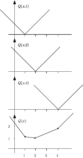
perplanes of Q(x) .

To see this, recall that Q(x)=E

Q(x,ξ)=

∑

k=1

Q(x,

) ,where

Q(x,

)=min{y

+ y

| y

−y

−x , y

≥ 0} .

In this very simple example, it is easy to see that if x ≤

, the second-stage optimal

solution is y

−x,0) while it is y

=(0,x −

) if x ≥

. Thus

Q(x,



−x if x ≤

x −

if x ≥

Figure 3 represents the functions Q(x,1) , Q(x,2) , Q(x,4) as well as Q(x) .

Now, consider again Iteration 1. x

= 0 is the starting point. Step 3 obtains the

cut

≥ 7/3 −x . From our construction, we see that, for x = x

, Q(x, 1)=1,

Q(x,2)=2, Q(x,4)=4andQ(x)=7/3 . But we can also conclude that “around

x = x

,” Q(x,1)=1 −x , Q(x, 2)=2 −x , Q(x,4)=4 −x and Q(x)=7/3 −x .

In fact, “around x = x

”issimply 0≤ x ≤ 1 . This can easily be seen from the

construction of Q(x,1) where Q(x,1) changes when x = 1 . In general, such a

range can be obtained by linear programming sensitivity analysis around the second-

stage optimal solutions.

We conclude that Q(x)=7/3 −x within 0 ≤ x ≤ 1 . The optimality cut at

the end of Iteration 1 is nothing other than

≥ 7/3 −x . It coincides with Q(x)=

190 5 Two-Stage Recourse Problems

Fig. 3 Recourse functions for Example 2.

7/3−x within 0 ≤x ≤1 and is a lower bound on Q(x) elsewhere (see Section 5.1

for the proof). We say that the optimality cut is a supporting hyperplane of Q(x) .

The L -Shaped algorithm successively adds four cuts which are supporting hy-

perplanes on the intervals [0,1] , [4,10] , [2,4] and [1,2] , respectively. Thus, at

the beginning of Iteration 5, a full description of Q(x) is available through the

four cuts. Obviously, such a full description is not needed. In fact, the optimum is

found here as soon as the supporting hyperplanes of the intervals [1,2] and [2,4]

are known. If, by chance, these two intervals were to be considered in the ﬁrst two

iterations, then two cuts (and three iterations) would sufﬁce to ﬁnd the optimum.

Thus, the efﬁciency of the L -Shaped algorithm can be inﬂuenced by an adequate

choice of the starting point.

Finally, observe that, by linear programming duality, the cuts (1.4) can also be

obtained from the primal second-stage solutions. Indeed, as we have seen in the

proof of Proposition 3 of Chapter 3, solving the second-stage program

5.1 The L -Shaped Method 191

Q(x,

)=min

{q(

)y |W(

)y = h(

) −T(

)x , y ≥ 0}

amounts to ﬁnding an optimal basis B(

) (a square submatrix of W ) such that

= B(

)

−1

(h(

) −T(

)x) , y

= 0andq

(

)

−1

. W ≤ q(

)

,where

and y

are the subvectors of y associated to the columns of B(

) andtothe

remaining columns, respectively. It follows that

Q(x,

)=q

(

)

·B(

)

−1

(h(

) −T(

)x) .

Sensitivity analysis shows that, for ﬁxed

, this relation holds for all x ’s such

that B(

)

−1

(h(

) −T(

)x) ≥ 0 . Noticing that

= q

(

)

·B(

)

−1

, one can

show that the cut (1.4) is identical to

≥ E

(

)

·B(

)

−1

(h(

) −T(

)x)}

and that the right-hand side of the cut coincides with Q(x) within

∩

∈

{x | B(

)

−1

(h(

) −T(

)x ≥0} .

The construction of the cuts from the primal second-stage solutions and the inﬂu-

ence of the starting point are further discussed in Exercise 2.

b. Feasibility cuts

Step2ofthe L -shaped method consists of determining whether a ﬁrst-stage deci-

sion x ∈ K

is also second stage feasible, i.e. x ∈ K

. This step can be done as

follows:

Step 2.For k = 1,...,K solve the linear program

min w



= e

+ e

−

(1.8)

s. t. Wy+ Iv

−Iv

−

= h

−T

y ≥0 , v

≥ 0 , v

−

≥ 0 ,

(1.9)

where e

=(1,...,1) , until, for some k , the optimal value w



> 0 . In this case,

let

be the associated simplex multipliers and deﬁne

r+1

)

(1.10)

and

r+1

)

(1.11)

to generate a constraint (called a feasibility cut)oftype(1.3). Set r = r + 1,addto

the constraint set (1.3), and return to Step 1. If for all k , w



= 0 , go to Step 3.

192 5 Two-Stage Recourse Problems

To illustrate the feasibility cuts, consider Example 4.2:

min 3x

+ 2x

−E

(15y

+ 12y

)

s. t. 3y

+ 2y

≤ x

+ 5y

≤ x

.8ξ

≤ y

≤ ξ

.8ξ

≤ y

≤ ξ

x,y ≥ 0 ,a.s.,

with ξ

= 4or6andξ

= 4 or 8 , independently, with probability 1/2 each and

ξ =(ξ

,ξ

)

To keep the discussion short, assume the ﬁrst considered realization of ξ is

(6,8)

. If not, many cuts would be needed. Starting from an initial solution

=(0,0)

, Program (1.8)–(1.9) reads as follows



= min v

+ v

−

+ v

−

+ v

−

+ v

−

+ v

−

+ v

−

s. t. v

−v

−

+ 3y

+ 2y

≤ 0 ,

−v

−

+ 2y

+ 5y

≤ 0 ,

−v

−

+ y

≥ 4.8 ,

−v

−

+ y

≥ 6.4 ,

−v

−

+ y

≤ 6 ,

−v

−

+ y

≤ 8 ,

−

,y ≥0

The optimal solution is w



= 11.2 with non-zero variables v

= 4.8and

= 6.4 . The corresponding dual variables are

=(−3/11,−1/11,1,1, 0,0) .

We observe that h =(0,0, 4.8, 6.4,6,8)

and that T consists of the two columns

(−1,0, 0,0,0, 0)

and (0,−1,0,0, 0,0)

; thus, D

=(−0.273, −0.091, 1,1,0, 0) .

T =(0.273,0.091) , while d

=(−0.273, −0.091,1,1,0,0) ·h = 11.2 , creating the

feasibility cut 3/11x

+ 1/11x

≥ 11.2or3x

+ x

≥ 123.2.

The ﬁrst-stage solution is then x

=(41.067,0)

. A second feasibility cut is

≥ 22.4. The ﬁrst-stage solution becomes x

=(33.6,22.4)

. A third feasibility

cut x

≥41.6 is generated. The ﬁrst-stage solution is:

=(27.2, 41.6)

which yields feasible second-stage decisions.

This example also illustrates that generating feasibility cuts by a mere application

of Step 2 of the L -shaped method may not be efﬁcient. Indeed, a simple look at the

problem reveals that, for feasibility when

= 6and

= 8 , it is at least necessary

to have y

≥ 4.8andy

≥ 6.4 , which in turn implies x

≥ 27.2andx

≥ 41.6.

5.1 The L -Shaped Method 193

We may then consider the following program as a reasonable initial problem:

min 3x

+ 2x

+ Q(x)

s. t. x

≥ 27.2 ,

≥ 41.6 ,

which immediately appears to be feasible. Such situations frequently occur in prac-

tice and are now discussed.

In some cases, Step 2 can be simpliﬁed. A ﬁrst case is when the second stage is

always feasible. The stochastic program is then said to have complete recourse. Let,

as in (1.1), the second-stage constraint be:

Wy = h −Tx, y ≥0 .

We repeat here the deﬁnition given in Section 3.1d. for complete recourse for con-

venience.

Deﬁnition. A stochastic program is said to have complete recourse when pos W =

ℜ

.Itissaidtohaverelatively complete recourse when K

⊇ K

, i.e., x ∈ K

implies h −Tx∈ pos W for any h, T realization of h,T .

If we consider the farmer’s problem in Section 1.1, program (1.1.2) has complete

recourse. The second stage just serves as a measure of the cost to the farmer of

the decisions taken. Any lack of production can be covered by a purchase. Any

production in excess can be sold. If we consider the power generation model (1.3.6),

it has complete recourse if there exists at least one technology with zero lead time

(

= 0) . If the demand in a given period t exceeds what can be delivered by the

available equipment, an investment is made in this (usually expensive) technology

to cover the needed demand.

A second case is when it is possible to derive some constraints that have to be sat-

isﬁed to guarantee second-stage feasibility. These constraints are sometimes called

induced constraints. They can be obtained from a good understanding of the model.

A simple look at the second-stage program in the example reveals the conditions

for feasibility. Constraints x

≥ 27.2andx

≥ 41.6 are examples of induced con-

straints. In the power generation model (1.3.6) of Section 1.3, the total possible

demand in a given stage t is obtained from (1.3.8)as

∑

j= 1

. The maximal possi-

ble demand in stage t is thus D

= max

∈

∑

j= 1

.Stage t feasibility will thus require

enough investments in the various technologies to cover the maximal demand, i.e.,

∑

i=1

t−

+ g

) ≥ D

Again, with the introduction of these induced constraints, Step 2 of the L -shaped

algorithm can be dropped.