Birge J.R., Louveaux F. Introduction to Stochastic Programming

Подождите немного. Документ загружается.

244 5 Two-Stage Recourse Problems

1 ≤ l ≤ j −1,

i, j

−h

i, j

and

i,l

= 0, l ≥ j + 1. If

< h

i,0

,thenlet

i,0

i,l

= 0,l ≥1 . In this way, we satisfy (7.3).

≥ h

i,1

,thevariable i objective term in (7.5) with these values is then

−q



i,1

j− 1

∑

l=1

i,l+1

−h

i,l

)+(

−h

i, j

)



+ q



j− 1

∑

l=1



(

∑

k=1

i,k

)(h

i,l+1

−h

i,l

)



∑

k=1

i,k

(

−h

i, j

)



= q

−q

+ q



j− 1

∑

k=1

i,k



j− 1

∑

l=k

i,l+1

−h

i,l

) −h

i, j



−p

i, j

∑

k=1

i,k



= q

−q

(

∑

k=1

i,k

)+q

(

∑

k=1

i,k

)

= q

−q



≤

dF(h

)+q

(

)

(

) , (7.6)

where the last equality follows from substitution in (7.2).

< h

i,1

, then the objective term is q

−q

which again agrees with

(

) from (7.2). Hence, any feasible (x,

) in (7.1) corresponds to a feasible

(x,

) (where

is extended into the components for each interval) in (7.5).

Suppose now that some (x

∗

) is optimal in (7.5). Because each q

> 0and

i, j

> 0,for h

i, j

≤

∗

< h

i, j+1

for some 1 ≤ j ≤ K

,wemusthave

∗

i,0

= h

i,1

∗

i,l

= h

i,l+1

−h

i,l

,1≤ l ≤ j −1,

∗

i, j

∗

−h

i, j

and

∗

i,l

= 0, l ≥ j + 1 . If not,

then

∗

i,l

< h

i,l+1

−h

i,l

−

for some l ≤ j −1and

∗

> 0forsome

l ≥

j + 1 . A feasible change of increasing

∗

i,l

and decreasing

∗

yields

an objective decrease of

∑

s=l+1

i,s

and would contradict optimality. Hence,

we must have that the i th objective term in (7.5)isagain

(

∗

) . Similarly, this

must be true if

∗

< h

i,1

. Therefore, any optimal solution in (7.1) corresponds to a

feasible solution with the same objective value in (7.5), and any optimal solution in

(7.5) corresponds to a feasible solution with the same objective value in (7.1). Their

optima must then correspond.

This formulation as an upper bounded variable linear program can lead to signiﬁ-

cant computational efﬁciencies. An implementation in Kallberg, White, and Ziemba

[1982] uses this approach in a short-term ﬁnancial planning model with 12 random

variables with three realizations, each corresponding to uncertain cash requirements

and liquidation costs. They solve the stochastic model with problem (7.5) in approx-

imately 1.5 times the effort to solve the corresponding mean value linear program

5.7 Simple and Network Recourse Problems 245

with expected values substituted for all random variables. This result suggests that

stochastic programs with simple recourse can be solved in a time of about the same

order of magnitude as a deterministic linear program ignoring randomness.

Further computational advantages for these problems are possible by treating the

special structure of the

i, j

variables as

variables with piecewise, linear convex

objective terms. Fourer [1985, 1988] presents an efﬁcient simplex method approach

for these problems. This implementation lends further support to the similar mean

value problem–stochastic program order of magnitude claim.

Decomposition methods can also be applied to the simple recourse problem with

ﬁnite distributions, although solution times better than the mean-value linear pro-

gramming solution would generally be difﬁcult to obtain. As mentioned in Sec-

tion 5.1d., the multicut approach offers some advantage for the L -shaped algorithm

(in terms of major iterations), but solution times are generally at best comparable

with the mean-value linear program time.

For generalized programming, because

(

∑

i=1

(

) and each

(

) is

easily evaluated, the subproblem in (6.10) is equivalent to ﬁnding

such that

−

∈

∂Ψ

(

) . (7.7)

From (7.4) and the argument in Proposition 5.1,

∂Ψ

(

)={d

i, j

} for h

i, j

i, j+1

and

∂Ψ

(

)=[d

i, j−1

i, j

] for h

i, j

. Thus, we can choose

= h

i, j

for d

i, j−1

≤−

≤ d

i, j

, j = 1,...,K

.If

< −q

, then the value in (6.10)is

unbounded. The algorithm chooses

s+1

= −1,and

0,i

(−1)=q

.Inthisway,

generalized programming can be implemented easily, but would appear similar to

the piecewise linear approach.

In network problems, the simple recourse formulation can be even more efﬁ-

ciently solved. Suppose, for example, that the random variables h

correspond to

random demands at m

destinations, that the variables x

are ﬂows from s to t ,

Ax = b corresponds to the network constraints for all source nodes, transshipment

nodes, and destinations with known demands, and that Tx represents all the ﬂows

entering the destinations with random demand. By adding the constraint,

∑

i=1



∑

j= 1

i, j



−

∑

sources s

∑

= −

∑

known demand

destinations r

demand(r) , (7.8)

every variable in (7.5) corresponds to a ﬂow so that (7.5) becomes a network linear

program. Hence, efﬁcient network codes can be applied directly to (7.5) in this case.

When T has gains and losses, (7.5) is a generalized network. This problem was

one of the ﬁrst types of practical stochastic linear programs solved when Ferguson

and Dantzig [1956] used the generalized network form to give an efﬁcient procedure

for allocating aircraft to routes (ﬂeet assignment). We describe this problem to show

the possibilities inherent in the stochastic program structure.

The problem includes m

aircraft and m

routes. The decision variables are

aircraft s allocated to route r . The number of aircraft s available is b

,the

passenger capacity of aircraft s on route r is t

, and the uncertain passenger

246 5 Two-Stage Recourse Problems

demand is h

. Hence, the i th row of Ax = b is

∑

r=1

= b

.The j -th row of

Tx−

= 0is

∑

s=1

−

= 0.

The key observation about this problem is that the basis corresponds to a pseudo-

rooted spanning forest (see, e.g., Bazaraa, Jarvis, and Sherali [1990]). For this prob-

lem, the simplex steps solve with trees and one-trees in an efﬁcient manner. For

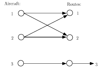
example, suppose m

= 3, m

= 3, b =(2,2, 2) , t

1·

=(200,100,300) , t

2·

(300,100,200) ,and t

3·

=(400,100,150) , p

i, j

= 0.5,and h

1,1

= 500 , h

1,2

= 700 ,

2,1

= 200 , h

2,2

= 400 , h

3,1

= 200 , h

3,2

= 400 . A basic solution is x

1,1

= 1,

1,2

= 1, x

2,1

= 1, x

2,2

= 1, x

3,3

= 2,and

3,1

= 100 with all other variables

nonbasic. This basis is illustrated in Figure 5. The forest consists of a cycle and a

subtree. Exercises 1, 2, and 3 explore this example in more detail.

Fig. 5 Graph of basic arcs for aircraft-route assignment example.

For general network problems, Sun, Qi and Tsai [1993] describe a piecewise linear

network method that allows the use of network methods and does not require adding

the additional arcs that correspond to the

i, j

values. Other generalizations for net-

work structured problems allow continuous distributions and apply directly to the

nonlinear problem. We discuss these methods in more detail in the next chapter.

The methods all apply to simple recourse problems in which the ﬁrst-stage vari-

ables represent a network. Another class of problems includes network constraints

in the second (and following) stages. These problems are called network recourse

problems. In this case, some computational advantages are again possible.

Most computational experience with solving these problems directly has been

with the L -shaped method. The efﬁciencies occur in constructing feasibility con-

straints, in generating facets of the polyhedral convex recourse function, and in solv-

ing multiple recourse problems using small Schur complement updates of a network

basis. These procedures are described in Wallace [1986b]. Other methods for net-

work recourse problems involve nonlinear programming-based procedures.

We suppose the simple recourse problem structure in (7.1). As noted earlier,

the most direct methods for solving (7.1) use standard nonlinear programming

techniques. We brieﬂy describe some of the alternatives here. The most com-

mon procedures applied here are single-point linearization approaches, such as the

5.7 Simple and Network Recourse Problems 247

Frank-Wolfe method, multiple-point linearization, such as generalized linear pro-

gramming as in Section 5.6, and active set or reduced variable methods, similar

to simplex method extensions. Other methods are described in Nazareth and Wets

[1986].

The Frank-Wolfe method for simple recourse problems appears in Wets [1966]

and Ziemba [1970]. The basic procedure is to approximate the objective using the

gradient and to solve a linear program to ﬁnd a search direction. The algorithm

contains the following basic steps. We assume that each random variable h

has an

absolutely continuous distribution function F

so that each

is differentiable. In

this case, the gradient of

(Tx) is easily calculated as ∇

(Tx)=(q

−q)

(

F)T ,

where

F = diag{F

i·

x)}, the diagonal matrix of the probability that h

is below

i·

x .

Frank-Wolfe Method for Simple Recourse Problems

Step 0. Suppose a feasible solution x

to (7.1). Let

= 0.GotoStep1.

Step 1.Let ˆx

solve:

min z =(c

+(q

−q)

(

)T)x

s. t. Ax = b ,

x ≥ 0 ,

(7.9)

where

= diag{F

i·

)}.

Step 2.Find x

to minimize c

( ˆx

−x

))+

∑

i=1

(T(x

( ˆx

−x

)))

over 0 ≤

≤ 1.If x

= x

, stop with an optimal solution. Otherwise, let

+ 1 and return to Step 1.

The basis for this approach is that x

∗

is optimal in (7.1) if and only if x

∗

solves

(7.9) with x

∗

= x

.If x

is not a solution of (7.1), then x

= x

, and descent

occurs along ˆx

−x

. Exercise 1 asks for the details of this convergence result.

The L -shaped method and generalized linear programming can be considered

extensions of the linearization approach that use multiple points of linearization.

We have already considered the L -shaped method in some detail in the previous

chapter. For generalized programming, the key advantage is that

(

) is separa-

ble. Williams [1966] and Beale [1961] observed the advantage of this property and

gave generalized programming procedures for speciﬁc problems. In the case of the

general problem in (7.1), the master problem of (3.4.9)–(3.4.10) becomes

min z

= c

x +

∑

j= 1



∑

i=1

0 j

(

∑

i=1

(

)



(7.10)

s. t. Ax = b , (7.11)

i·

x −

∑

i=1

−

∑

i=1

= 0 , j = 1,...,m

, (7.12)

248 5 Two-Stage Recourse Problems

∑

i=1

= 1 , (7.13)

≥ 0 , i = 1,...,r

;

≥ 0 , i = 1,...,s

, j = 1,...,m

where we can divide the components of

in the constraints because of the separa-

bility.

We then have a subproblem of the form in (3.5.12) for each j :

min

(

−

. (7.14)

We can create an entering column whenever any of the values in (7.14) is negative.

If all are non-negative, then the algorithm again terminates with an optimal value.

Example 4

As an example of generalized programming applied to a simple recourse problem,

suppose the following situation. We have $400 to buy boxes of blueberries ($5 per

box) and cherries ($7 per box) from a farmer. We take the berries to the town market

where we hope to sell them ($11 per blueberry box and $15 per cherry box). Any

unsold berries at the end of the market day can be sold to a local baker ($3 per

blueberry box and $5 per cherry box).

The demand for berries is stochastic. We assume that blueberry demand dur-

ing market hours is uniformly distributed between 10 and 30 boxes and that cherry

demand is uniformly distributed between 20 and 40 boxes. In the simple recourse

problem, the correlation between these demands does not affect the recourse func-

tion value; so, we only need this marginal information.

The initial decisions are x

, the number of boxes of blueberries to buy, and x

the number of boxes of cherries to buy. The full problem is then to ﬁnd x

∗

min z = 2x

+ 2x

(

)

s. t. 5x

+ 7x

≤ 400 ,

−

= 0 ,

−

= 0 ,

≥ 0 ,

(7.15)

where

(

⎧

⎪

⎨

⎪

⎩

−8

≤ 10 ,

−12

+ 20 if 10 ≤

≤ 30 ,

−160 if

≥ 30 ,

5.7 Simple and Network Recourse Problems 249

∇

(

⎧

⎪

⎨

⎪

⎩

−8if

≤ 10 ,

−12 if 10 ≤

≤ 30 ,

0if

≥ 30 ,

(

⎧

⎪

⎨

⎪

⎩

−10

≤ 20 ,

−20

+ 100 if 20 ≤

≤ 40 ,

−300 if

≥ 40 ,

and

∇

(

⎧

⎪

⎨

⎪

⎩

−10 if

≤ 20 ,

−20 if 20 ≤

≤ 40 ,

0if

≥ 40 .

The generalized programming method follows these iterations.

Iteration 0:

Step 0. We start with (7.10)–(7.13) with

= r

= s

= 0.

Step 1. The obvious solution is x

=(0,0)

with multipliers,

=(0,0)

Step 2. Setting

=−∇

(

) , we obtain

= 30 and

= 40 with

(

−160 and

(

)=−300 and clearly

(

j,s

−

< 0 for each

j = 1,2.Now, s

= s

= 1,

= 1 and we repeat.

Iteration 1:

Step 1. We assume that we can dispose of berries (to avoid creating an infeasibility

in (7.10)–(7.13)). The master problem then has the form:

min z = 2x

+ 2x

−160

−300

s. t. 5x

+ 7x

≤ 400 ,

−30

≥ 0 ,

−40

≥ 0 ,

= 1 ,

≥ 0 .

(7.16)

The solution is z

= −300 , x

=(24,40)

= 0.8,

= 1.0,

=(5.333,

6.667)

and

=(0,−33.333)

Step 2. Setting

= −∇

(

) , we obtain

= 16.667 and

= 26.667 with

(

)=−124.4and

(

)=−255.55 . Again,

(

j,s

−

< 0 for each j = 1, 2 with

(

−

= −35.5and

(

−

= −44.4.Now, s

= s

= 2,

= 2.

250 5 Two-Stage Recourse Problems

Iteration 2:

Step 1. The new master problem is:

min z = 2x

+ 2x

−160

−124.4

−300

−255.55

s. t. 5x

+ 7x

≤ 400 ,

−30

−16.667

≥ 0 ,

−40

−26.667

≥ 0 ,

= 1 ,

≥ 0 .

(7.17)

The solution is z

= −316.0, x

=(24, 40)

= 0.55 ,

= 0.45 ,

= 1.0,

=(2.667,2.934)

and

=(−80.0,− 182.6)

Step 2. Setting

= −∇

(

i,s

) , we obtain

= 23.33 and

23 = 34.13 with

(

)=−151.1and

(

)=−291.4.Here,

(

−

= −8.88

and

(

−

= −8.61 . Now, s

= s

= 3,

= 3.

Iteration 3:

Step 1. The new master problem is:

min z = 2x

+ 2x

−160

−124.4

−151.1

−300

−255.55

−291.4

s. t. 5x

+ 7x

≤ 400 ,

−30

−16.667

−23.333

≥ 0 ,

−40

−26.667

−34.133

≥ 0 ,

= 1 ,

≥ 0 .

(7.18)

The solution is z

= −327.57 , x

=(23.333,34.133)

= 1.00 ,

= 1.0,

=(2.0,2.0)

and

=(−104.44,−223.13)

Step 2. Setting

= −∇

(

i,s

) , we obtain

= 25 and

24 = 36 with

(

)=−155 and

(

)=−296 . Here,

(

−

= −0.56 and

(

−

= −0.87 . Now, s

= s

= 4,

= 3.

Iteration 4:

5.7 Simple and Network Recourse Problems 251

Step 1.Weadd

and

with their objective and constraint entries to (7.18)to

obtain the same form of the master problem. The solution is now z

= −329 , x

(25,36)

= 1.00 ,

= 1.0,

=(2.0,2.0)

and

=(−105,−224)

Step 2. Because

, we obtain

,and

(

−

= 0for

i = 1,2 . Hence, no columns can be added. We stop with the optimal solution, x

∗

(25,36)

with objective value z

∗

= 329 .

Notice that in this example the budget constraint is not binding. We only spend

$377 of the total possible, $400. If we had solved this problem as separate news

vendor problems in each type of berry, we would have obtained the same solution.

In fact, this is one of the suggestions for initial tenders to start the generalized pro-

gramming process (see Birge and Wets [1984] and Nazareth and Wets [1986]). In

this case, we would terminate on the ﬁrst step with this initial offer (just as in the

case of Example 2 described in Section 5.6).

Notice also as in Section 5.6 that the algorithm appears to converge quite quickly

here. In general, the retention of information about gradients at many points should

improve convergence over techniques that use only local information. Second-

order information is also valuable, assuming twice-differentiable functions. This

is the motivation behind Beale’s [1961] approach of quadratic approximation. This

method is another form of the generalized programming approach for convex sepa-

rable functions.

The other procedures speciﬁcally used on the simple recourse problem concern

some form of active set or simplex based strategy. Wets [1966] and Ziemba [1970]

give the basic reduced gradient or convex simplex method procedure. This method

consists of computing a search direction corresponding to a change in the value of a

nonbasic variable (assuming only basic variables change concomitantly). The basis

is changed if the line search implies that basic variable becomes zero. Otherwise,

the nonbasic variable’s value is updated and other nonbasic variables are checked

for possible descent.

A different approach is given by Qi [1986], who suggests alternating between

the solution of a linear program with

ﬁxed and the solution of a reduced variable

convex program. The linear program is to ﬁnd

min

x +

(

)

s. t. Ax = b ,

Tx=

x ≥ 0 ,

(7.19)

to obtain x

=(x

) ,where x

= 0 . Then solve the reduced convex program:

min

x +

(

)

s. t. Ax = b , Tx=

≥ 0 , x

= 0,

(7.20)

252 5 Two-Stage Recourse Problems

to obtain ˆx

. The algorithm is the following.

Alternating Algorithm for Simple Recourse Problems

Step 0.Let

= 0 , choose a feasible solution x

to (7.20)andlet

be part of a

solution to (7.20) with N deﬁned according to x

.GotoStep1.

Step 1.Solve(7.19). Let X

= {x optimal in (7.19) } . Choose x

∈X

such

that c

(Tx

) < c

(Tx

) . If none exists, then stop. Otherwise,

go to Step 2.

Step 2.Solve(7.20) with N deﬁned for x

to obtain

.Let

+ 1and

return to 1.

The algorithm converges to an optimal solution because x

can always be

found with c

(Tx

) < c

(Tx

) whenever x

is not optimal

(Exercise 5). Of course, the algorithm’s advantage is when the number of ﬁrst-period

variables n

is much greater than the number of second-period random variables

, so that solving problem (7.20) provides a computational savings over solving

(7.1) directly.

This algorithm (and indeed the convex simplex method) raises the possibility for

multiple optima of the linear program (degeneracy). In this case, many solutions

may be searched before improvement is found. In tests of partitioning in discretely

distributed general stochastic linear programming problems (Birge [1985b]), this

problem was found to overcome computational advantages of reducing the working

problem size. The approach has, therefore, not been followed extensively in practice

although it may, of course, offer efﬁcient computation on some problems.

Other methods for simple recourse have built on the special structure. For trans-

portation constraints, Qi [1985] gives a method based on using the forest structure

of the basis to obtain a search direction and improved forest solution. This method

only requires the solution of one-dimensional monotone equations apart from stan-

dard tree solutions. Piecewise linear techniques as in Sun, Qi, and Tsai [1990] can

also be adapted here to general network structures and used in conjunction with Qi’s

forest procedure to produce a convergent algorithm.

Exercises

1. Show that any basis for the aircraft allocation problem consists of a collection of

+ m

basic variables that correspond to a collection of trees and one-trees.

2. Describe a procedure for ﬁnding the values of basic variables, multipliers, re-

duced costs, and entering and leaving basic variables for the structure in the

aircraft allocation problem.

3. Solve the aircraft allocation problem using the procedure in (7.2) starting at

the basis given with cost data corresponding to c

1·

=(300,200, 100) , c

2·

5.8 Methods Based on the Stochastic Program Lagrangian 253

(400,100,300) , c

3·

=(200,100,300) , q

= 25 , q

−

= 0foralli .Youmay

ﬁnd it useful to use the graph to compute the appropriate values.

4. Show that the Frank-Wolfe method for the simplex recourse problem converges

to an optimal solution (assuming that one exists).

5. Solve the example in (7.15)usingthe L -shaped method.

6. Solve the example in (7.15) using the Frank-Wolfe method.

7. In the general stochastic linear programming model (with ﬁxed T ,(3.1.5)),

show that solving (7.19) with

∗

yields an optimal solution x

∗

.Use

this to show that there always exists a solution to (3.1.5) with at most m

+ m

nonzero variables (Murty [1968]). What does this imply for retaining cuts in the

L -shaped method?

8. Show that the alternating algorithm for simple recourse problems converges to

an optimal solution assuming that the support of h is compact. (Hint:From any

, consider a path to x

∗

, use the convexity of

, and consider the solution as

is approached from x

∗

5.8 Methods Based on the Stochastic Program Lagrangian

Again consider the general nonlinear stochastic program given in (3.5.1), which we

repeat here without equality constraints to simplify the following discussion:

infz = f

(x)+Q(x) (8.1)

s. t. g

(x) ≤ 0 , i = 1,...,m

where Q(x)=E

[Q(x,

)] and

Q(x,

)=inf f

(y(

) (8.2)

s. t. g

(x,y(

) ≤ 0 , i = 1,...,m

with the continuity assumptions mentioned in Section 3.5.

In general, we can consider a variety of approaches to (8.1) based on available

nonlinear programming methods. For example, we may consider gradient projec-

tion, reduced gradient methods, and straightforward penalty-type procedures, but

these methods all assume that gradients of Q are available and relatively inexpen-

sive to acquire. Clearly, this is not the case in stochastic programs because each

evaluation may involve solving several problems (8.2). Lagrangian approaches have

been proposed to avoid this problem.

The basic idea behind the Lagrangian approaches is to place the ﬁrst- and second-

stage links into the objective so that repeated subproblem optimizations are avoided

in ﬁnding search directions. To see how this approach works, consider writing (8.1)

in the following form: