Birge J.R., Louveaux F. Introduction to Stochastic Programming

Подождите немного. Документ загружается.

274 6 Multistage Stochastic Programs

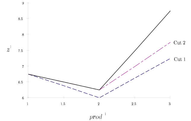
In Figure 1, the solid line gives the objective value in (1.7) as a function of total

production prod

= x

+ w

in the ﬁrst period. The dashed lines correspond to the

cuts made by the algorithm (Cut 1,2). The ﬁrst cut was 2.25y

≥ 5.75 from

(1.15)–(1.16) on Iteration 2. Because y

= x

+ w

−1 , we can substitute for y

to obtain, 2.25x

+ 2.25w

≥ 8 . The objective in (1.17)is z

= x

+ 3w

0.5y

, so, combined with 1 ≤ x

≤ 2 , we can substitute

≥ 8 −2.25(prod

)

to obtain z

(prod

)=7.5 +(1.5) min{2, prod

}+ 3.5(prod

−2)

−2.25prod

where prod

≥ 1 . This can also be written as:

(prod



7.5 −0.75prod

if prod

≤ 2 ,

3.5 + 1.25prod

if prod

> 2 ,

(1.18)

which corresponds to the wide dashed line (Cut 1) in Figure 1.

Fig. 1 The ﬁrst period objective function (solid line) for the example and cuts (dashed lines) gen-

erated by the nested L -shaped method.

The second cut occurs on Iteration 4 (verify this in Exercise 2) as 2x

+ 2w

≥

7.75 , which yields z

(prod

)=x

+3w

+0.5y

≥7.25+(1.5)min{2, prod

3.5(prod

−2)

−2prod

(prod

) ≥



7.25 −0.5prod

if prod

≤ 2 ,

3.25 + 1.5prod

if prod

> 2 .

(1.19)

This cut corresponds to the narrow width dashed line (Cut 2) in Figure 1.

6.1 Nested Decomposition Procedures 275

The optimal value and solution in terms of prod

can be read from Figure 1 as

each cut is added. With only Cut 1, the lowest value of z

occurs when prod

= 2.

With Cuts 1 and 2, the minimum is also achieved at prod

= 2 . Note that the ﬁrst

cut is not, however, a facet of the objective function’s graph. The cuts meet the

objective at prod

= 1andprod

= 2 , respectively, but they need not even do

this, as we mentioned earlier (see Exercise 3). The other parts of the Period 1 cuts

are generated from bounds on Q

This example illustrates some of the features of the nested L -shaped method.

Besides our not being guaranteed of obtaining a support of the function at each step,

another possible source of delay in the algorithm’s convergence is degeneracy. As

the example illustrates, the solutions at each step occur at the links of the piecewise

linear pieces generated by the method (Exercises 5 and 5). At these places, many

bases may be optimal so that several bases may be repeated. Some remedies are

possible, as in Birge [1980] and, for deterministic problems, Abrahamson [1983].

As with the standard two-stage L -shaped method, the nested L -shaped method

acquires its greatest gains by combining the solutions of many subproblems through

bunching (or sifting). In addition, multicuts are valuable in multistage as well as

two-stage problems. Infanger [1991, 1994] has also suggested the uses of generat-

ing many cuts simultaneously when future scenarios all have similar structure. This

procedure may make bunching efﬁcient for periods other than H by making ev-

ery constraint matrix identical for all scenarios in a given period. In this way, only

objective and right-hand side constraint coefﬁcients vary among the different sce-

narios.

In terms of primal decomposition, we mentioned the work of No¨el and Smeers

at the outset of this chapter. They apply nested Dantzig-Wolfe decomposition to the

dual of the original problem. As we saw in Chapter 5, this is equivalent to applying

outer linearization to the primal problem. The only difference is that they allow for

some nonlinear terms in their constraints, which would correspond to a nonlinear

objective in the primal model. Because the problems are still convex, nonlinearity

does not really alter the algorithm. The only problem may be in the ﬁniteness of

convergence.

The advantage of a primal or dual implementation generally rests in the problem

structure, although primal or dual simplex may be used in either method, making

them indistinguishable. Gassmann [1990] presents some indication that dual iter-

ations may be preferred in bunching. In general, many primal columns and few

rows would tend to favor a primal approach (outer linearization as in the L -shaped

method) while few columns and many rows would tend to favor a dual approach.

In any case, the form of the algorithm and all proofs of convergence apply to either

form.

While nested decomposition (and other linearization methods) are particularly

well-suited for linear problems, the general methods apply equally well for con-

vex nonlinear problems (i.e., problems with convex, time-separable objectives and

convex constraints, see Exercise 8). Birge and Rosa [1996] describe a nested de-

composition of this form applied to global energy-economy-environmentinteraction

276 6 Multistage Stochastic Programs

models. They use an active set approach for the subproblems, but interior point

methods might also be used.

Exercises

1. Verify that the infeasibility condition is as given in Step 1 of the nested L -

shaped method. (Hint: note that if x

satisﬁes (1.2)and(1.3), then there exists

such that (x

) satisfy (1.4).)

2. Continue Example 1 with the nested L -shaped method until you obtain an op-

timal solution.

3. Construct a multistage example in which a cut generated by the second period

in following the nested L -shaped method does not meet Q

) for any value

of x

,i.e., −E

+ e

< Q(x

) .

4. Show that the situation in (1.1) is not possible if the fast-forward protocol is

always followed.

5. Suppose a feasibility cut (1.3) is active for x

for any t and k . Show that

every basic feasible solution of NLDS(t +1, j) with input x

for some scenario

j ∈ D

t+1

(k) must be degenerate.

6. Suppose two optimality cuts (1.4) are active for (x

) for any t and k .Show

that either the subproblems generate a new cut with

or an optimal

solution of NLDS(t + 1, j) with input x

for some scenario j ∈D

t+1

(k) must

be degenerate.

7. Using four processors, what efﬁciency can be gained by solving the preceding

example in parallel? Find the utilization of each processor and the speed-up of

elapsed time, assuming each subproblem requires the same solution time.

8. Suppose

is broken into separate components for Q

and Q

as in the two-

stage multicut approach. How does that alter the solution of the example?

9. Suppose that the objective in each period t for each scenario k is a general

convex function f

t−1

) and, in addition to the linear constraints, there is

an additional convex constraint, g

t−1

) ≤0 . Assuming relatively complete

recourse for simplicity and that your solver can return the primal solution and

dual multipliers for the K-K-T system of equations, describe how you would

modify the nested decomposition steps to accommodate these nonlinear func-

tions.

6.2 Quadratic Nested Decomposition

Decomposition techniques for multistage nonlinear programs are available for the

case in which the objective function is quadratic convex, the constraint set polyhe-

6.2 Quadratic Nested Decomposition 277

dral, and the random variables discrete. For the sake of clarity, we repeat the recur-

sive deﬁnition of the deterministic equivalent program, already given in Section 3.4.

(MQSP) min z

)=(c

)

+(x

)

+ Q

)

s. t. W

= h

≥0 ,

(2.1)

where Q

t−1

(

)) =

min (c

(

))

(

)+(x

(

))

(

)+Q

t+1

)

s. t. W

(

)=h

(

) −T

t−1

(

t−1

(

) ≥ 0 ,

(2.2)

t+1

)=E

t+1

(

)) , t = 1,...,H −1 , (2.3)

and

H−1

)=0 . (2.4)

In MQSP , D

is an n

×n

matrix. All other matrices have the dimensions

deﬁned in the linear case. The random vector,

(

) , is formed by the elements of

(

) , h

(

) , T

t−1

(

) ,and D

(

) . We keep the notation that ξ

is an N

-vector

on (

,P) , with support

. Finally, we again deﬁne

= {x

| Q

t+1

) < ∞} .

We also deﬁne z

)=(c

)

+(x

)

+ Q

t+1

) .

Theorem 2. If the matrices D

(

) are positive semi-deﬁnite for all

∈

and t = 1,...,H , then the sets K

and the functions Q

t+1

) are convex for

t = 1,...,H −1 .If

is also ﬁnite for t = 2,...,H,then K

is polyhedral. More-

over z

) is either identically −∞ or there exists a decomposition of K

into a

polyhedral complex such that the t

-stage deterministic equivalent program (2.2)

is a piecewise quadratic program.

Proof: The piecewise quadratic property of (2.2) is obtained by inductively apply-

ing to each cell of the polyhedral complex of K

the result that if z

(·) is a ﬁnite

positive semi-deﬁnite quadratic form, there exists a piecewise afﬁne continuous op-

timal decision rule for (2.2). All others results were given in Section 3.4.

We now describe a nested decomposition algorithm for MQSP ﬁrst presented in

Louveaux [1980]. For simplicity in the presentation of the algorithms, we assume

relatively complete recourse. This means that we skip the step that consists of gener-

ating feasibility cuts. If needed, those cuts are generated exactly as in the multistage

linear case. We keep the notation of a(k) for the ancestor scenario of k at stage

278 6 Multistage Stochastic Programs

t −1 . As in Section 6.1, c

, D

,and Q

t+1

represent realizations of c

, D

,and

t+1

for scenario k and x

is the corresponding decision vector. In Stage 1, we

use the notations, z

and z

and x

, as equivalent.

Nested PQP Algorithm for MQSP

Step 0.Set t = 1, k = 1, C

= S

= K

. Choose x

∈ K

Step 1.If t = H ,gotoStep2.For i = t + 1,...,H ,let k = 1, z

)=(c

)

and C

i−1

a(1)

)=S

i−1

a(1)

)=K

i−1

a(1)

) . Choose x

∈ K

i−1

a(1)

) .Set t =

H .

Step 2.Find v ∈ argmin{z

) | x

∈ S

t−1

a(k)

)}.Find w ∈ argmin{z

) | x

∈

t−1

a(k)

)}.If w is the limiting point on a ray on which z

(·) is decreasing to −∞ ,

then (DEP)

is unbounded and the algorithm terminates.

Step 3.If ∇

(w)(v −w)=0 , go to Step 4. Otherwise, redeﬁne

t−1

a(k)

) ← S

t−1

a(k)

) ∩{x

| ∇

(w)(x

−w) ≤ 0} .

Let x

= v , z

=(c

)

+(x

)

and C

= K

t−1

a(k)

) .GotoStep1.

Step 4.If t = 1 , stop; w is an optimal ﬁrst-period decision. Otherwise, ﬁnd the cell

t−1

a(k)

) containing w and the corresponding quadratic form Q

t−1

a(k)

) . Redeﬁne

t−1

a(k)

t−1

a(k)

) ← z

t−1

a(k)

t−1

a(k)

)+p

t−1

a(k)

)

t−1

a(k)

t−1

a(k)

) ←C

t−1

a(k)

t−1

a(k)

) ∩G

a(k)

t−1

) .

If k = K

,let t ←t −1 , go to Step 2. Otherwise, let k ←k+1, z

)=(c

)

, C

= S

t−1

a(k)

)=K

t−1

a(k)

) . Choose x

∈S

t−1

a(k)

) .GotoStep1.

Theorem 3. The nested PQP algorithm terminates in a ﬁnite number of steps by

either detecting an unbounded solution or ﬁnding an optimal solution of the multi-

stage quadratic stochastic program with relatively complete recourse.

Proof: The proof of the ﬁnite convergence of the PQP algorithm in Section 5.3

amounts to showing that Step 2 of the algorithm can be performed at most a ﬁnite

number of times. The same result holds for a given piecewise quadratic program

(2.2) in the nested sequence. The theorem follows from the observations that there

is only a ﬁnite number of different problems (2.2) and that all other steps of the

algorithm are ﬁnite.

Numerical experiments are reported in Louveaux [1980]. It should be noted that

the MQSP easily extends to the multistage piecewise convex case. The limit there

is that the objective function and the description of the cell are usually much more

difﬁcult to obtain. One simple example is proposed in Exercise 3.

6.2 Quadratic Nested Decomposition 279

It is interesting to observe that the MQSP method has a tendency to require few

iterations when the quadratic terms play a signiﬁcant role and a good starting point is

chosen. (This probably relates to the good behavior of regularized decomposition.)

Example 1 (continued)

Assume that the cost of overtime is now quadratic (for example, larger increases

of salary are needed to convince more people to work overtime). We replace ev-

erywhere 3.0w

by 2.0w

+(w

)

. Assume all other data are unchanged. Take as

the starting point a situation where 0 ≤ y

≤ 1, 0≤ y

≤ 1, k = 1,2 . (It is rela-

tively easy to see what the corresponding values for the other ﬁrst- and second-stage

variables should be.) We now proceed backward. Let t = 3.

i) t = 3, k = 1.Wesolve

min x

+ 2w

+(w

)

s. t. y

+ x

+ w

= 1 , x

≤ 2 ,

≥ 0 ,

where inventory at the end of Period 3 has been omitted for simplicity. The solution

is easily seen to be x

= 1 −y

, w

= 0 and is valid for 0 ≤ y

≤1 . It follows that

)=1−y

ii) t = 3, k = 2.Wesolve

min x

+ 2w

+(w

)

s. t. y

+ x

+ w

= 3 , x

≤ 2 ,

≥ 0 .

The solution is now x

= 2, w

= 1 −y

, valid for 0 ≤y

≤1 . It yields Q

4 −2y

+(1 −y

)

Combining (i) and (ii), we obtain

−

(1 −y

)

and

)={y

| 0 ≤ y

≤ 1} .

iii) and iv) Because the randomness is only in the right-hand side, we conclude

that cases (iii) and (iv) are identical to (i) and (ii), respectively. Hence,

−

(1 −y

)

and C

)={y

| 0 ≤ y

≤ 1} .

280 6 Multistage Stochastic Programs

Next, we have t = 2.

i) t = 2, k = 1 . The objective z

is computed as

= x

+ 2w

+(w

)

+ 0.5y

−

(1 −y

)

i.e.,

+ x

+ 2w

+(w

)

−y

(1 −y

)

The constraint sets are

= {x

| y

+ x

+ w

−y

= 1 , 0 ≤x

≤ 2 , x

≥ 0}

and

= S

∩{0 ≤y

≤ 1} .

The solution v of minimizing z

(·) over S

= 1 , x

= 2 −y

Because the solution belongs to C

, we can take w = v .(Bewarethat w without

superscript and subscript corresponds to the optimal solution on a cell deﬁned in

Step 2, while w with superscript and subscript corresponds to overtime.) Thus, this

point satisﬁes the optimality criterion in Step 3. It yields

+ 2 −y

−1 =

−y

and

)={y

| 0 ≤ y

≤ 2} .

ii) t = 2, k = 2 . The objective z

is similarly computed as

+ x

+ 2w

+(w

)

−y

(1 −y

)

The constraint set

= {x

| y

+ x

+ w

−y

= 3 , 0 ≤x

≤ 2 , x

≥ 0}

only differs in the right-hand side of the inventory constraint with

= S

∩{0 ≤y

≤ 1} .

The solution v is now x

= 2, w

= 1−y

= 0.Again v ∈C

,sothatwehave

w = v , which satisﬁes the optimality criterion in Step 3. It yields

6.2 Quadratic Nested Decomposition 281

+ 2 + 2(1 −y

)+(1 −y

)

= 7 −2y

+(1 −y

)

and

)={y

| 0 ≤ y

≤ 1} .

Next is the case for t = 1.

The current objective function is computed as

= 21/4 −y

(1 −y

)

+ x

+ 2w

+(w

)

The constraint sets are

= {x

| x

+ w

−y

= 1 , x

≤ 2 , x

≥ 0} ,

= S

∩{0 ≤y

≤ 1} .

The solution v of minimizing z

over S

= 2 , y

= 1 , w

= 0 ,

with objective value z

. Because this solution belongs to C

, it is the optimal

solution of the problem. Thus, no cut was needed to optimize the problem.

Exercises

1. Consider Example 1 with quadratic terms as in this section and take 1 ≤y

≤2,

1 ≤ y

≤ 2, 0≤ y

≤ 1 as a starting point. Show that the following steps are

generated. Obtain 0.5Q

)+0.5Q

−

.In t = 2, k = 1 , solution

v is x

= 0, y

= y

−1 while w is y

= 1, x

= 2 −y

, both with w

= 0.

Acut x

+ 2w

≤

−y

is added. The new starting point is v ,which

corresponds to 0 ≤y

≤1 . Then the case t = 2, k = 1 is as in the text, yielding

−y

and C

)={0 ≤y

≤ 2} .

In t = 2, k = 2 (see the calculations in the text), we obtain Q

)=6 −y

and C

)={1 ≤y

≤3}.Thus,in t = 1, z

= x

+2w

+(w

)

−y

and C = {1 ≤ y

≤ 2}. Again, the solution v : x

= 1, y

= 0, w

= 0 does

not coincide with w : x

= 2, y

= 1, w

= 0.Acut x

−

+ w

≤ 3/2is

generated. The new starting point now coincides with the one in the text and the

solution is obtained in one more iteration.

282 6 Multistage Stochastic Programs

6.3 Block Separability and Special Structure

The deﬁnition of block separability was given in Section 3.4. It permits separate

calculation of the recourse functions for the aggregate level decisions and the de-

tailed level decisions. This is an advantage in terms of the number of variables and

constraints, but often it makes the computation of the recourse functions and of

the cells of the decomposition much easier in the case of a quadratic multistage

program. This has been exploited in Louveaux [1986] and Louveaux and Smeers

[2011].

We will illustrate a further beneﬁt. It also consists of separating the random vec-

tors. Consider the production of a single product. Now, assume the product cannot

be stored (as in the case of a perishable good) or that the policy of the ﬁrm is to use

a just-in-time system of production so that only a ﬁxed safety stock is kept at the

end of each period.

Assume that units are such that one worker produces exactly one product per

stage. Two elements are uncertain: labor cost and demand. Labor cost is currently 2

per period. Next period, labor cost may be 2 or 3 , with equal probability. Current

revenue is 5 per product in normal time and 4 in overtime. Overtime is possible

for up to 50% of normal time. Demand is a uniform continuous random variable

within (0,200) and (0,100) , respectively, for the next two periods. The original

workforce is 50 . Hiring and ﬁring is possible once a period, at the cost of one unit

each. Clearly, the labor decision is the aggregate level decision.

To keep notation in line with Section 3.4, we consider a three-stage model. In

Stage 1, the decision about labor is made, say for Year 1. Stage 2 consists of pro-

duction of Year 1 and decision about labor for Year 2. Stage 3 only consists of

production of Year 2. Let

be labor cost in stage t , while

is the demand in

stage t .Let w

be the workforce in stage t . Then,

t−1

,ξ

)=min|w

−w

t−1

|+ ξ

+ Q

t+1

) , (3.1)

t+1

)=E

t+1

,ξ

t+1

)+Q

t+1

,ξ

t+1

)] , (3.2)

and Q

t+1

,ξ

t+1

) is minus the expected revenue of production in stage t + 1

given a workforce w

and a demand scenario ξ

t+1

. It is obtained as follows.

Let D

represent the maximal demand in stage t ( 200 for t = 2 , 100 for t =

3 ). Observe that the expectation of ξ

is D

/2 because ξ

is uniformly continuous

over [0,D

] .If w

≥D

, all demand can be satisﬁed with normal time. If w

≤D

≤

1.5w

, demand up to w

is satisﬁed with normal time, the rest in overtime. Finally,

if D

≥1.5w

, normal time is possible up to a demand of w

, overtime from w

1.5w

, and extra demand is lost. Taking expectations over these cases, we obtain

t+1

)=E

t+1

)] =

⎧

⎪

⎨

⎪

⎩

−2.5D

if w

≥ D

)

−w

−2D

if w

≤ D

≤1.5w

5(w

)

−7w

if 1.5w

≤ D

6.3 Block Separability and Special Structure 283

This problem can now be solved with the MQSP algorithm. Assume w

= 50 ,

≥ 50 .

Let Stage (2, 1) represent the ﬁrst labor scenario in Stage 2, i.e.,

= 2.The

problem consists of ﬁnding

min |w

−w

|+ 2w

+ Q

)

s. t. w

≥ 0 .

We compute Q

)=Q

5(w

)

100

−7w

,for w

≤

200

, because D

= 100 .

We also replace |w

−w

| by an explicit expression in terms of hiring (h

) and

ﬁring ( f

). The problem in Stage (2,1) now reads:

,1)=min h

+ f

−5w

5(w

)

100

s. t. w

−h

+ f

= w

≥ 0 , h

≥ 0 , f

≥ 0 .

Under this form, the problem is clearly quadratic convex (remember w

is w in

Stage 2, not the square of w ). Classical Karush-Kuhn-Tucker conditions give the

optimal solution w

= w

, as long as 40 ≤ w

≤ 60 . Then

,1)=−5w

5(w

)

100

Similarly, in Scenario (2, 2) where

= 3 , the solution of

min |w

−w

|+ 3w

+ Q

)

s. t. w

≥ 0

is w

= 50 , f

= w

−50 , as long as w

≥ 50 . Then

,2)=w

−125 ,

and

)=−

125

−2w

2.5(w

)

100

which is valid within C

= {50 ≤w

≤ 60}.

The Stage 1 objective is:

min h

+ f

+ 2w

+ Q

)+Q

so that the Stage 1 problem reads:

min h

+ f

−7w

)

−

125