Biringen S., Chow C.-Y. An Introduction to Computational Fluid Mechanics by Example

Подождите немного. Документ загружается.

102 INVISCID FLUID FLOWS

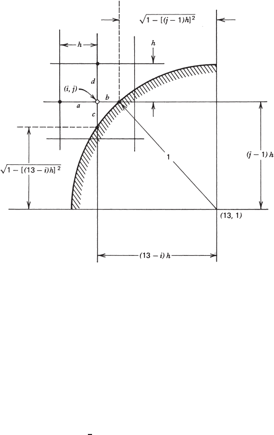
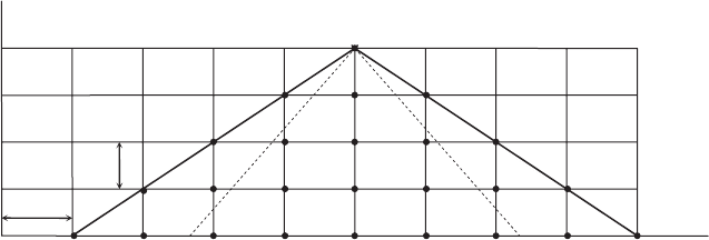
FIGURE 2.9.5 Agridpoint(i, j) near the left surface of the circular cylinder.

Next we consider the derivative boundary condition that ∂ψ/∂x = 0atthe

exit. By using the central-difference formula (2.2.8), the condition becomes

i+1, j

= ψ

i−1, j

for i = 25 and j = 2, ..., 8 (2.9.9)

This suggests that an additional column of ﬁctitious grid points is needed at a

distance h to the right of the exit section, as indicated in Fig. 2.9.3. These ﬁctitious

points do not show speciﬁcally in the computation, because with substitution of

(2.9.9) the iterative formula (2.9.3) at i = 25 becomes

i, j

)

2ψ

i−1, j

+ψ

i, j −1

+ψ

i, j +1

(2.9.10)

In summary, there are three types of grid points besides the boundary points:

(1) the points in the close neighborhood of the cylinder, (2) those at the exit

section of the channel, and (3) the remaining grid points inside the ﬂuid. To

classify the type, we introduce an identiﬁcation number

ID at each of the interior

points and assign to it the integer value of 1, −1, or 0 according to the location

of that point as speciﬁed in the order just mentioned.

After the numerical solution for ψ has been obtained, the ﬂow pattern is

plotted following the same procedure as that described in Program 2.6. The ﬂow

POTENTIAL FLOWS IN DUCTS OR AROUND BODIES 103

0.1

0.9

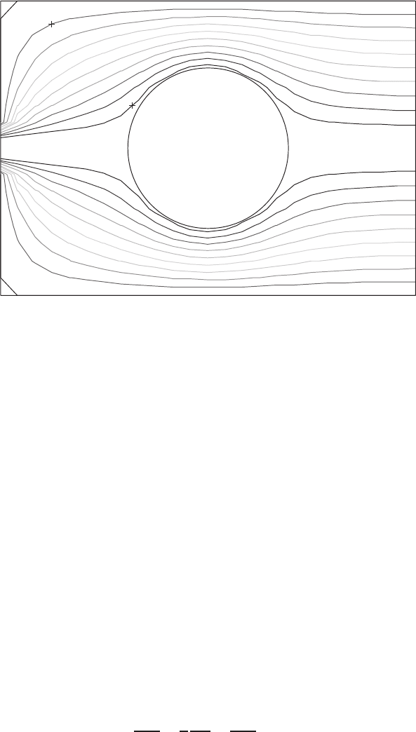
FIGURE 2.9.6 Channel ﬂow past a circular cylinder.

pattern below the centerline of the channel is the mirror image of that above. In

the program listing, we also provide an alternative way of plotting selected ψ

values by the use of MATLAB contour plotting routines.

Most of the variable names used in Program 2.7 are exactly the same as those

used in Program 2.6. New names are listed as follows:

ID, A, B, C,andD have

just been deﬁned, and

JFIRST(I) is the value of j at the lowest interior grid point

on the ith grid line.

The output of Program 2.7, Fig. 2.9.6, shows that the ﬂow speed on the right

side of the cylinder is slower than that on the left. The pressure difference has a

tendency to push the body upstream.

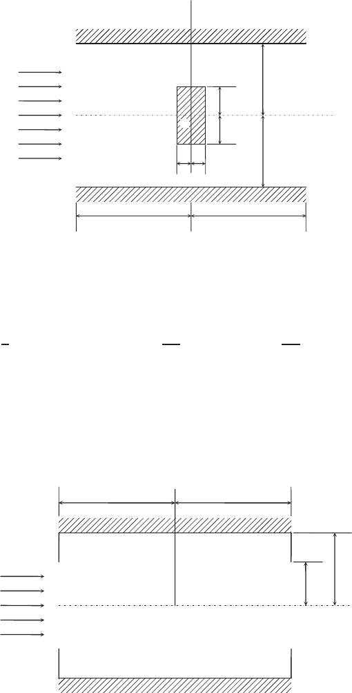
Problem 2.9 Compute and plot the channel ﬂow past a cylinder of rectangular

cross section shown in Fig. 2.9.7. The potential ﬂow pattern is assumed to be

symmetric about both the x and y axes, so that only the upper left quarter of

the ﬂow needs to be computed. It is further assumed that the ﬂow entering the

section AB is approximately uniform and the speed there is unity.

The boundary conditions are that ψ = 0 along AFED, ψ = 1 along BC , ψ =

y/4 along AB,and∂ψ/∂x = 0 along CD. In the computation let h = 0.25.

Problem 2.10 The equation governing the stream function of an axisymmetric

potential ﬂow was derived previously as (2.6.2) having the form

∂

∂r

−

∂ψ

∂r

∂

∂z

= 0

104 INVISCID FLUID FLOWS

FIGURE 2.9.7 Channel ﬂow past a rectangular cylinder.

Show that for a square mesh of size h, this partial differential equation may be

solved numerically by using the following iterative formula:

i, j

i−1, j

+ψ

i+1, j



1 +



i, j −1



1 −



i, j +1

(2.9.11)

where r

is the radial distance of point (i, j ) from the z axis. Using this

numerical scheme, compute and then plot the ﬂow in the region bounded by

OABCDO within an axisymmetric tube containing repeated partitions (see

Fig. 2.9.8). Choose a square mesh of size h = 0.1 for numerical computation.

0.5

FIGURE 2.9.8 Axisymmetric ﬂow through a tube containing repeated partitions.

NUMERICAL SOLUTION OF HYPERBOLIC PARTIAL DIFFERENTIAL EQUATIONS 105

Around the boundary of this region, ψ = 0 along OD, ψ = 1 along ABC ,and

∂ψ/∂z = 0 along both OA and CD. The derivative boundary conditions are the

result of symmetry of stream function about these two sections.

2.10 NUMERICAL SOLUTION OF HYPERBOLIC PARTIAL

DIFFERENTIAL EQUATIONS

Problems concerning wave motions in ﬂuid mechanics are governed by hyper-

bolic partial differential equations. One example mentioned in Section 2.7 is the

supersonic ﬂow past a thin body whose governing equation is (2.7.2). Another

commonly cited example is the propagation of a one-dimensional sound wave of

small amplitude, described by (see Liepmann and Roshko, 1957, p. 68)

∂

∂t

= a

∂

∂x

(2.10.1)

in which t is time, x is the coordinate in the direction of wave propagation, a is

the speed of sound treated as constant in the linearized analysis, and u is the ﬂuid

speed. It can be shown that density, pressure, and temperature are all governed

by equations of the same form.

In this section a numerical technique is developed for solving (2.10.1) to ﬁnd

u at any time t > 0 in the spatial domain 0 ≤ x ≤ L, provided that the initial

conditions of u are given at t = 0 and are expressed in the following form, with

functions f and g to be speciﬁed for a particular problem:

u(x,0) = f (x) (2.10.2)

∂u

∂t

(x,0) = g(x) (2.10.3)

Boundary conditions are to be speciﬁed at both ends of the gaseous domain, say

within a channel of constant cross-sectional area. If one end of the channel is

enclosed by a rigid wall, then u must be zero there at all times. On the other hand,

at an end that opens to the atmosphere, the pressure there must be a constant or,

alternatively, ∂u/∂x must vanish at that section.

To solve this mixed initial-boundary-value problem numerically, we divide

the spatial range of the domain into small intervals of length h and the time axis

into intervals of size τ . The total number of vertical grid lines is m, whereas that

of horizontal grid lines can be as many as needed in a particular computation.

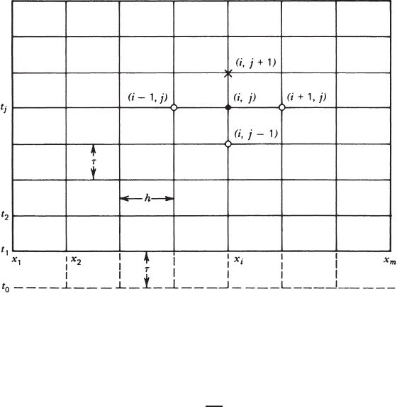
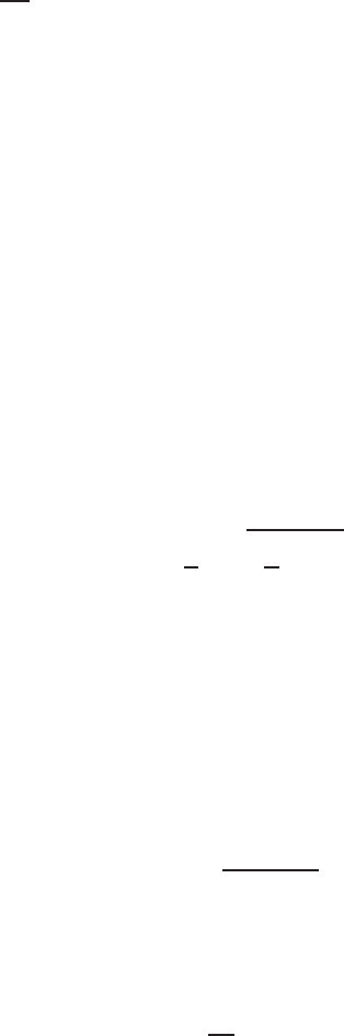
Lines and points in the grid system are named according to Fig. 2.10.1.

A difference equation can be derived following exactly the same procedure as

that used to obtain the numerical scheme (2.8.2) for solving the Poisson equation.

Using the central-difference formula to approximate the derivatives in (2.10.1),

we obtain, after regrouping,

i, j +1

= 2u

i, j

)

i−1, j

−2u

i, j

i+1, j

−u

i, j −1

(2.10.4)

106 INVISCID FLUID FLOWS

FIGURE 2.10.1 Grid system for numerical computation.

where C is a dimensionless parameter called the Courant number,deﬁnedby

C =

aτ

(2.10.5)

(2.10.4) computes the solution at a certain time level based on the solutions at

two previous time levels.

Actually, various numerical schemes can be constructed for solving the same

partial differential equation by using different ﬁnite-difference approximations.

In Section 2.13, we will introduce a multistep explicit method, the MacCormack

explicit method (1969), which can be easily extended to nonlinear hyperbolic

systems. The applicability of a numerical scheme is determined by whether it

is stable, that is, whether the numerical solution grows and becomes unbounded

after repeatedly applying the scheme. In a way, we have proved in Section 2.8 that

Richardson’s iterative formula is stable, and so is Liebmann’s. Here we will use a

different approach to ﬁnd the conditions under which (2.10.4) is computationally

stable. It turns out that the stability of this numerical scheme is determined by

the magnitude of C .

Following von Neumann’s stability analysis, we assume that time and space

variables are separable and that the solution to (2.10.4) can be expanded in the

form of a Fourier series. A representative Fourier component may be written

i, j

= U

Iikh

(2.10.6)

NUMERICAL SOLUTION OF HYPERBOLIC PARTIAL DIFFERENTIAL EQUATIONS 107

where U

is the amplitude at t

of the wave component whose wave number is

k,andI =

√

−1. Similarly,

i, j ±1

= U

j±1

Iikh

, u

i±1, j

= U

I (i±1)kh

Substituting these into (2.10.4) gives, after canceling the common factor e

Iikh

j+1

= 2U

−Ikh

Ikh

−2) −U

j−1

By using the identity that (e

I θ

−I θ

)/2 = cos θ, it becomes

j+1

= AU

−U

j−1

(2.10.7)

where A ≡ 2[1 −C

(1 − cos kh)]. By introduction of an ampliﬁcation factor λ

such that

= λU

j−1

and U

j+1

= λU

= λ

j−1

(2.10.8)

(2.10.7) is reduced to

−Aλ + 1 = 0 (2.10.9)

whose roots are

λ =





−1 (2.10.10)

For |A|≥2, the roots are real, but their magnitudes are |λ|≥1; for |A| < 2

the magnitudes of the complex roots are equal to 1. An inspection of (2.10.8) con-

cludes that the amplitude grows indeﬁnitely with increasing time unless |λ|≤1.

Thus, the inequality that |A|≤2orA

≤ 4 determines the condition for stability;

that is, for stability,

[1 − C

(1 − cos kh)]

≤ 1

After expanding the left side and rearranging, we obtain

≤

1 − cos kh

When cos kh varies from −1to+1, the function on the right-hand side varies

from 1 to inﬁnity, of which the lowest value is chosen to insure stability. There-

fore, the stability criterion for the numerical scheme (2.10.4) is C

≤ 1, or

aτ

≤ 1 (2.10.11)

To arrive at this expression, we have used the fact that each of the three variables

on its left is positive. This relationship implies that τ and h cannot be chosen

independently.

108 INVISCID FLUID FLOWS

If the Courant number is chosen to be

aτ

= 1 (2.10.12)

then (2.10.4) takes an especially simple form:

i, j +1

= u

i−1, j

i+1, j

−u

i, j −1

(2.10.13)

As shown in Fig. 2.10.1, this equation states that the value of u at a grid

point marked by a cross is computed from the values already computed at

three circled grid points at two previous time steps. The numerical scheme

(2.10.13) is commonly referred to as the leapfrog method. It will now be proved

that this numerical method actually gives the exact solution to the differential

equation (2.10.1).

It is well known that the solution to (2.10.1) satisfying initial conditions

(2.10.2) and (2.10.3) is

u(x, t) =



f (x + at) + f (x − at)



x+at

x−at

g(v) dv (2.10.14)

which can be veriﬁed by substituting it back into each of those equations. The

solution may be written in the simpler functional form

u(x, t) = F (x − at) +G(x +at) (2.10.15)

where the functions F and G represent simple waves propagating without chang-

ing shape along the positive and negative x directions at constant speed a.The

lines of slope dx/dt =±a in the x − t plane, which trace the progress of the

waves, are called the characteristics of the wave equation (see Liepmann and

Roshko, 1957, p. 69).

When applied at a grid point (x

, t

), (2.10.15) becomes

i, j

= F(x

−at

) +G(x

+at

)

From Fig. 2.10.1 we have

= x

+(i −1)h and t

= t

+(j − 1)τ

so that

i, j

= F(α +ih −jaτ) + G(β +ih + jaτ)

in which α ≡ (x

−h) −a(t

−τ) and β ≡ (x

−h) +a(t

−τ). With aτ = h,

obtained from the condition that C = 1, it reduces to

i, j

= F



α + (i − j )h





β +(i +j )h



NUMERICAL SOLUTION OF HYPERBOLIC PARTIAL DIFFERENTIAL EQUATIONS 109

According to this relation, the right-hand side of (2.10.13) is rewritten

i−1, j

i+1, j

−u

i, j −1

= F



α + (i − j −1)h







β +(i +j − 1)h







α +(i −j + 1)h





β +(i +j + 1)h



−F





α +(i −j + 1)h



−G





β +(i +j − 1)h



= F[α +(i −j − 1)h] +G[β +(i +j + 1)h]

which is exactly u

i, j +1

or the left-hand side of (2.10.13). It follows that the exact

solution is computed for (2.10.1) by the leapfrog scheme (2.10.13).

Having introduced the concept of characteristics, we are now in a position

to interpret the physical meaning of the stability criterion (2.10.11) by use of

Fig. 2.10.2. An examination of (2.10.4) reveals that the solution at the grid point

P is inﬂuenced by the solution at each of the grid points at previous time steps

contained within two diagonals PQ and PR of slope (dx/dt)

=±h/τ . Thus, the

region PQRP is the domain of dependence of point P in the numerical computa-

tion. If Pq and Pr are the backward characteristics of slope (dx/dt)

=±a pass-

ing through P,andifa < h/τ or, equivalently, if then |(dx/dt)

| < |(dx/dt)

these lines will lie between PQ and PR, as shown in the ﬁgure. However, from

the theory of characteristics, it is known that point P can receive signals only

from the region PqrP, which is its physical domain of dependence. In the present

case of aτ/h < 1, in which the computational domain of dependence contains

the physical domain of dependence, all the information required to determine

the condition at P is included in the computation so that the numerical scheme

is stable. The result is inaccurate because of the inclusion of some unneces-

sary information originating from the region between PQ and Pq and the region

between PR and Pr.Ifaτ/h > 1, the characteristics Pq and Pr would be drawn

outside of PQ and PR. In this case only a part of the needed information is

used to determine the solution at P, and the computation is unstable. It becomes

Rqr

FIGURE 2.10.2 Physical interpretation of the stability criterion (2.10.11).

110 INVISCID FLUID FLOWS

obvious that when aτ/h = 1 (i.e., when the computational and physical domains

of dependence coincide), the numerical solution is the exact solution.

In using the formula (2.10.13) information is needed at two previous time

steps. It cannot be used directly at the initial stage to compute the solution at t

since conditions are speciﬁed only at the initial instant t

= 0. To help start the

numerical procedure, we construct in Fig. 2.10.1 a row of ﬁctitious grid points

= t

−τ , and then rewrite the initial conditions (2.10.2) and (2.10.3) in index

notation:

i,1

= f

(2.10.16)

i,0

= u

i,2

−2τ g

(2.10.17)

in which f

and g

represent, respectively, f (x

) and g(x

). In obtaining the second

expression we have approximated ∂u/∂t by the central-difference form (2.2.8).

For j = 1 and with substitution from the preceding equations, (2.10.13) becomes

i,2

= u

i−1,1

i+1,1

−u

i,0

= f

i−1

i+1

−u

i,2

+2τg

i,2

i−1

i+1

) + τ g

, i = 2, ..., m − 1 (2.10.18)

This is called the starting formula for (2.10.13).

2.11 PROPAGATION AND REFLECTION

OF A SMALL-AMPLITUDE WAVE

Although exact solutions of the linear partial differential equation (2.10.1) can

be written out in the form of (2.10.14), the work is still tedious when waves

interact or reﬂect from boundaries. In this section these phenomena are examined

numerically by using the leapfrog method just derived.

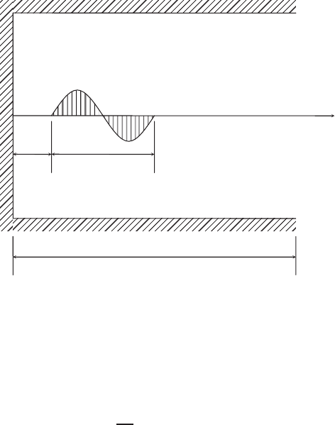
We consider a one-dimensional tube 1 m in length, with the left end closed

and the right end open (Fig. 2.11.1). At t = 0 a sinusoidal wavelet of 0.4-m

wavelength is somehow generated in the tube at a distance 0.2 m from the left

end. Let the amplitude of the wavelet be 1 m/s, and let the functions f and

g used in (2.10.2) and (2.10.3) to describe the initial conditions be deﬁned as

follows:

f (x) = sin



2π

x −0.2

0.4



for 0.2 ≤ x ≤ 0.6 (2.11.1)

= 0elsewhere

g(x) = 0for0≤ x ≤ 1 (2.11.2)

PROPAGATION AND REFLECTION OF A SMALL-AMPLITUDE WAVE 111

0.2 m 0.4 m

x = 0

u(x,0)

FIGURE 2.11.1 Sinusoidal wavelet in a one-dimensional tube.

The boundary conditions are

u(0, t) = 0 (2.11.3)

∂u

∂x

(1, t) = 0 (2.11.4)

Under sea level conditions, the speed of sound is a = 340 m/s.

For numerical computation we choose h = 0.02 m, so that the number of

vertical grid lines is m = 51 and the space occupied initially by the wavelet is

between grid lines 11 ≤ i ≤ 31. Thus, the nonvanishing f

values for these values

of i are given by

= sin

{

5π

[

(i − 1)h −0.2

]

}

(2.11.5)

and g

= 0 for all values of i.

The boundary condition (2.11.3) when written in index notation is

1, j

= 0forallj (2.11.6)

To handle the condition (2.11.4), which contains a derivative with respect to

x, we construct a column of ﬁctitious grid points in the x-t plane along the

grid line i = m +1, in the same fashion as shown in Fig. 2.9.3. Consequently,