Biringen S., Chow C.-Y. An Introduction to Computational Fluid Mechanics by Example
Подождите немного. Документ загружается.

232 NUMERICAL SOLUTION OF THE INCOMPRESSIBLE NAVIER-STOKES EQUATION
of vorticity at x
m
during a time period τ is, according to (4.2.2),
ζ
m, j +1
−ζ
m, j
=−
uτ
h
( − 0) =−
uτ
h
(4.2.14)
The change at x
m+1
, which is a point one grid downstream from x
m
, during the
same period is calculated also from (4.2.2) as
ζ
m+1, j +1
−ζ
m+1, j
=−
uτ
h
(0 −) =+
uτ
h
(4.2.15)
The result shows that the perturbation is transported, as it should be, from one
point to another in the downstream direction. It is also concluded that the numer-
ical solution to the differential equation (4.2.1) based on (4.2.3) is exact if uτ/h,
or C, is chosen to be unity.
Problem 4.2 Using an approximation with forward differencing in time and
central differencing in space, (4.2.1) is replaced by the finite-difference equation
ζ
i, j +1
= ζ
i, j
−
1
2
C (ζ
i+1, j
−ζ
i−1, j
) (4.2.16)
Use the discrete perturbation stability analysis to show that stability of this numer-
ical scheme can be achieved only when C → 0. Show also that (4.2.16) does
not possess the transportive property.
The upwind differencing scheme (4.2.2) is now reexamined from a different
point of view. Expanding its first and last terms in the form of a Taylor series
about the value of ζ
i, j
we obtain
ζ
i,j+1
= ζ
i,j
+τ
∂ζ
∂t
i,j
+
1
2
τ
2
∂
2
ζ
∂t
2
i,j
+O(τ
3
) (4.2.17)
ζ
i−1,j
= ζ
i,j
−h
∂ζ
∂x
i,j
+
1
2
h
2
∂
2
ζ
∂x
2
i,j
+O(h
3
) (4.2.18)
Substituting into (4.2.2) and dropping the subscripts i and j gives
∂ζ
∂t
+
τ
2
∂
2
ζ
∂t
2
+O(τ
2
) =−u
∂ζ
∂x
+
1
2
uh
∂
2
ζ
∂x
2
+O(h
2
) (4.2.19)
The second term on the left side can be evaluated for constant u from (4.2.1) as
∂
2
ζ
∂t
2
=
∂
∂t
−u
∂ζ
∂x
=−u
∂
∂x
∂ζ
∂t
= u
2
∂
2
ζ
∂x
2
(4.2.20)
Upon substitution of this expression in (4.2.19) and with terms up to the first
order in τ and h retained, the differential equation
∂ζ
∂t
+u
∂ζ
∂x
= μ
e
∂
2
ζ
∂x
2
(4.2.21)
UPWIND DIFFERENCING AND ARTIFICIAL VISCOSITY 233
is obtained in which
μ
e
=
1
2
uh(1 −C ) (4.2.22)
is a constant determined by the grid size τ and h. Because the term on the right-
hand side of (4.2.21) is caused by the errors inherited when (4.2.1) is replaced by
(4.2.2), and because this term is analogous to the diffusive viscous force term in
the Navier-Stokes equation (3.1.7), the coefficient μ
e
is called the artificial vis-
cosity. Its effect is to introduce artificial damping and diffusion in the numerical
solution. μ
e
vanishes when either C = 1 or both τ and h approach zero. Under
that condition, (4.2.21) reverts to the original differential equation (4.2.1).
Hirt (1968) argued that the effect of a diffusion term is to smear out a dis-
turbance in ζ so that a negative diffusion coefficient is physically impossible,
or otherwise the opposite would happen. The requirement that μ
e
≥ 0 results in
C ≤ 1, which is the stability criterion (4.2.13) derived previously for the upwind
numerical scheme (4.2.3). The present procedure for determining the stability,
based on a differential equation constructed from the finite-difference equation
through Taylor series expansion, is called Hirt’s stability analysis.
Problem 4.3 Applying Hirt’s stability analysis to the explicit formula (3.5.3)
for solving parabolic equation (3.5.1), show that the resulting differential
equation is
∂u
∂t
= ν
∂
2
u
∂y
2
+
1
2
νh
2
1
6
−R
∂
4
u
∂y
4
(4.2.23)
by retaining terms up to O(τ , h
2
),inwhichR = ντ/h
2
. Positive terms of even
derivatives, like the second-order derivative term, cause damping. Thus, the sta-
bility condition R ≤
1
6
so obtained is more restrictive than the condition R ≤
1
2
obtained in Section 3.5 using von Neumann’s stability analysis.
Show also that when Hirt’s stability analysis is applied to the implicit formula
(3.6.1), the same conclusion is deduced that the numerical scheme is stable for
any positive value of R.
Problem 4.4 Show that by using the discrete perturbation stability analysis,
the condition R ≤
1
2
is obtained for (3.5.3) in agreement with von Neumann’s
method.
The results stated in Problems 4.4 and 4.5 indicate that a stability criterion
deduced from the discrete perturbation stability analysis or from Hirt’s stability
analysis may or may not agree with that deduced from von Neumann’s analysis.
The reason for the disagreement is that the condition for computational stability
in each analysis is derived based on a different physical argument. Both von
Neumann’s and the discrete perturbation analyses require that the amplitude of
a disturbance should not grow with time. But the former is concerned with a
distribution of disturbances that can be synthesized by a Fourier series, whereas
the latter traces only the influence of a point perturbation. Hirt’s stability condition
is based on the fact that a diffusion coefficient cannot be negative. Despite the
234 NUMERICAL SOLUTION OF THE INCOMPRESSIBLE NAVIER-STOKES EQUATION
fact that von Neumann’s stability analysis is most commonly used, each method
has its own advantages as well as limitations. A comparison and evaluation of
these three methods can be found in Chapter 3, Section A-5, of Roache (1972).
By using a model equation (4.2.1), we have shown that the substantial deriva-
tive may be approximated by the upwind differencing scheme, which is compu-
tationally stable if the ratio τ/h is chosen appropriate for the local fluid velocity.
Furthermore, the upwind differencing scheme introduces, in addition to the trun-
cation errors, an artificial diffusion whose effect is to smear out perturbations in
the numerical solution. For thorough referencing and a more detailed discussion
on the subject and its related topics, Sections A-8 to A-11 in Chapter 3 of Roache
(1972) are recommended.
4.3 B
´
ENARD AND TAYLOR INSTABILITIES
When a horizontal layer of fluid is heated from below in a gravitational field, the
density of the fluid at any location becomes smaller than the fluid just above it.
If a fluid parcel is displaced slightly upward into the region of higher density, a
buoyant force will assist it to move further upward. Similarly, if the fluid parcel
is displaced downward into a region of smaller density, it will keep moving
in the same direction. Without a sufficiently large, viscous, retarding force, this
situation is said to be unstable, and the instability appears in the form of a net
of hexagonal convection cells.
Lord Rayleigh (1916) made the first theoretical analysis of the so-called
B´enard problem concerning the stability of a fluid layer in the presence of a tem-
perature gradient parallel to the gravitational force. An extensive treatment on this
subject based on linearized theories can be found in the book by Chandrasekhar
(1961). An example of a solution procedure for the linearized equations for his
problem was presented in Section 3.8 of this book. As we have observed there, the
linearized theory predicts only the onset of instabilities. Once the flow becomes
unstable, the initially small disturbances will grow with time, and the subsequent
fluid motion will be governed by the nonlinear Navier-Stokes equation. Now that
we already have a successful upwind-difference numerical scheme for approxi-
mating the nonlinear terms in that equation, the method used in Section 4.2 will
be adopted here to study the B
´
enard problem numerically on the computer.
The governing equations for the fluid motion are (3.1.1) to (3.1.3), the conti-
nuity, the Navier-Stokes (adding the buoyant force), the energy equations, and,
also, the equation of state. For the last equation we use, instead of (3.1.5), the
following form:
ρ = ρ
0
1 − α(T −T
0
)
(4.3.1)
where α is the coefficient of volume expansion and T
0
is the temperature at which
the fluid density is ρ
0
. For ordinary gases or liquids, α is of the order of 10
−3
or 10
−4
. Based on this fact, considerable simplifications can be made by using
the Boussinesq approximation that, if temperature variations are not too large, ρ
B
´
ENARD AND TAYLOR INSTABILITIES 235
can be considered constant everywhere except in the buoyant force term. Under
further assumption of constant physical properties of the fluid, (3.1.1) and (3.1.2)
become
∇ · V = 0 (4.3.2)
ρ
0
DV
Dt
=−j(ρ −ρ
0
)g − ∇p +μ∇
2
V (4.3.3)
in which j is the unit vector along the y-axis opposite to the direction of the
gravitational acceleration g. It can be shown (see Section II.8, Chandrasekhar,
1961) that the energy equation (3.1.3) reduces to
DT
Dt
= κ∇
2
T (4.3.4)
where κ(= k/ρ
0
c
v
) is the coefficient of thermometric conductivity, and c
v
is
the constant-volume specific heat. Note that the dissipation function drops out
completely from the energy equation in the present approximation.
We consider a two-dimensional flow in the x-y plane contained between two
flat plates at y = 0andy = H , respectively. The fluid originally at a uniform
temperature T
0
is heated from below by increasing the temperature of the lower
plate suddenly to T
1
. Being perpendicular to the fluid motion, the vorticity is in
the z direction and its magnitude is designated ζ . Again, a stream function ψ
can be introduced to satisfy (4.3.2).
For this problem H is a reference length, μ/ρ
0
H is a reference velocity, and
T
1
−T
0
is a reference temperature difference. Based on these reference quantities,
the following dimensionless variables are constructed:
X =
x
H
, Y =
y
H
, T =
t
ρ
0
H
2
/μ
U =
u
μ/ρ
0
H
, V =
v
μ/ρ
0
H
, =
ψ
μ/ρ
0
, (4.3.5)
=
ζ
μ/ρ
0
H
2
, θ =
T −T
0
T
1
−T
0
From now on T is used to designate the dimensionless time, and θ is used to
designate the dimensionless temperature difference.
Density difference in (4.3.3) is first replaced by temperature difference, with
substitution from (4.3.1). Then the pressure gradient term is eliminated after tak-
ing the curl of the resulting equation of motion. When expressed in dimensionless
form, the governing equations are
U =
∂
∂Y
(4.3.6)
V =−
∂
∂X
(4.3.7)
236 NUMERICAL SOLUTION OF THE INCOMPRESSIBLE NAVIER-STOKES EQUATION
=−
∂
2
∂X
2
+
∂
2
∂Y
2
(4.3.8)
∂
∂T
+
∂(U )
∂X
+
∂(V )
∂Y
= Gr
∂θ
∂X
+
∂
2
∂X
2
+
∂
2
∂Y
2
(4.3.9)
∂θ
∂T
+
∂(U θ)
∂X
+
∂(V θ)
∂Y
= Pr
−1
∂
2
∂X
2
+
∂
2
∂Y
2
θ (4.3.10)
in which Gr = αgH
3
(T
1
−T
0
)/ν
2
is the Grashof number and Pr = ν/κ is the
Prandtl number, ν(= μ/ρ
0
) being the kinematic viscosity coefficient. In some
analyses the Rayleigh number instead of the Grashof number is used, which is
defined as the product of Gr and Pr. The nonlinear terms in (4.3.9) and (4.3.10)
are written in the same form, so that both equations can be solved by using the
same numerical technique.
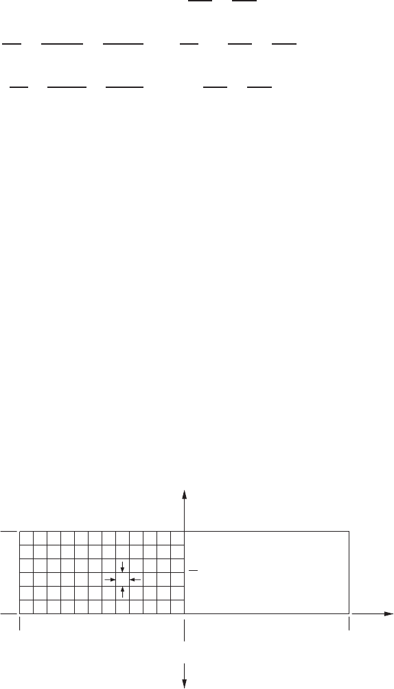
In Program 4.2 we consider water (Pr = 6.75) enclosed by a rectangular box,
shown schematically in Fig. 4.3.1. Because of the symmetry about the Y axis,
only the left half of the flow needs to be computed, thus resulting in large
savings in computational efforts. Square meshes of size h ×h are chosen for the
numerical work, and the concerned fluid region is covered with m vertical and n
horizontal grid lines. Since the dimensionless distance between parallel plates is
unity, the grid size h has the value of 1/(n –1). The values m = 21 and n = 9
are assumed for the present example.
At time T = 0, the temperature distribution is such that θ = 0everywhere,
except θ = 1 on the lower plate. As time increases, fluid temperature changes,
but the values at solid walls are kept always at the initial condition. The bound-
ary condition along the Y axis is ∂θ/∂X = 0, as required by the symmetry
of the temperature field. The temperature boundary conditions are indicated in
Fig. 4.3.1.
j = 1
h
i = m
X
Y
j = n
i = 1
g
θ = 1, ψ = 0
∂θ
∂x
= 0, ψ = 0
θ = 0, ψ = 0
θ = 0, ψ = 0
FIGURE 4.3.1 Schematic representation of the problem considered in Program 4.2.
B
´
ENARD AND TAYLOR INSTABILITIES 237
Except the nonlinear terms, all spatial derivatives in the governing differential
equations are approximated at the interior grid points using the central-difference
formula. The finite-difference forms of (4.3.6) and (4.3.7) are
U
i,j
=
i,j+1
−
i,j−1
2h
(4.3.11)
V
i,j
=−
i+1,j
−
i−1,j
2h
(4.3.12)
Equation (4.3.8) conforms with the generalized Poisson equation (2.8.1) if is
replaced by f and − by q. The successive overrelaxation method represented
by the iterative scheme (2.8.13) is programmed in the subroutine
SORLX,which
is used to find the stream function for a certain known vorticity distribution.
The maximum error
ERRMAX allowed in our program for the SOR method is
0.0001. The boundary conditions for stated in this subroutine are those shown
in Fig. 4.3.1, specified particularly for the present problem. The condition that
= 0 on the three solid walls comes from the fact that there is no net flow
across these boundaries. must also vanish along the Y axis to make the fluid
motion to its right the mirror image of that to its left. When the same subroutine
is used elsewhere, care must be taken to check whether the boundary conditions
need to be modified accordingly.
The symmetric distribution of θ and the antisymmetric distribution of about
the Y axis result in the following boundary conditions for all values of j :
θ
m+1, j
= θ
m−1, j
(4.3.13)
m, j
= 0 (4.3.14)
m+1, j
=−
m−1, j
(4.3.15)
U
m+1, j
=−U
m−1, j
(4.3.16)
U
m, j
= 0 (4.3.17)
V
m, j
=
m−1, j
h
(4.3.18)
m,j
= 0 (4.3.19)
The last three conditions are deduced from (4.3.11), (4.3.12), and (4.3.8), respec-
tively, by using (4.3.14) and (4.3.15).
To solve both (4.3.9) and (4.3.10), a function subprogram named
PNEW is
constructed for handling a generalized equation of the form
∂P
∂T
=−
∂(UP)
∂X
−
∂(VP)
∂Y
+A
∂Q
∂X
+B
∂
2
P
∂X
2
+
∂
2
P
∂Y
2
(4.3.20)
The computationally stable upwind-differencing scheme of the previous section
is used to approximate the first two terms on the right-hand side of this equation.
238 NUMERICAL SOLUTION OF THE INCOMPRESSIBLE NAVIER-STOKES EQUATION
Here, we adopt a solution method developed by Torrance (1968) for solving
natural correction (Torrance and Rockett, 1969) and rotating flow (Kopecky and
Torrance, 1973) problems. We first define U
f
and U
b
as the average x-directional
velocities evaluated, respectively, at half a grid point forward and backward from
the point (X
i
, Y
j
) in the x direction, given as
U
f
=
1
2
(U
i+1,j
+U
i,j
)
U
b
=
1
2
(U
i,j
+U
i−1,j
)
(4.3.21)
and, similarly, for V
V
f
=
1
2
(V
i,j+1
+V
i,j
)
V
b
=
1
2
(V
i,j
+V
i,j−1
)
(4.3.22)
Further defining,
P1 = (U
f
−|U
f
|)P
i+1, j
+(U
f
+|U
f
|−U
b
+|U
b
|)P
i, j
−(U
b
+|U
b
|)P
i−1, j
(4.3.23)
P2 = (V
f
−|V
f
|)P
i, j +1
+(V
f
+|V
f
|−V
b
+|V
b
|)P
i, j
−(V
b
+|V
b
|)P
i, j −1
(4.3.24)
the upwind differencing form is preserved. The terms multiplied by A and B are
approximated by central-differencing schemes. For them we let
P3 = Q
i+1, j
−Q
i−1, j
(4.3.25)
P4 = P
i+1, j
+P
i−1, j
+P
i, j +1
+P
i, j −1
−4P
i, j
(4.3.26)
Finally, a forward-differencing scheme is used to approximate the time derivative,
so that
∂P
∂T
i, j
=
1
T
(P
i, j
−P
i, j
) (4.3.27)
in which T is the size of the time increment and a prime is used to denote
the value of a variable evaluated at time T + T . Thus, after rearranging terms,
(4.3.20) becomes
P
i, j
= P
i, j
+
T
2h
−P1 −P2 +A ·P3 + 2B
P4
h
(4.3.28)
When (4.3.28) is used to integrate (4.3.9) at an interior grid point, we replace P
by , Q by θ,andletA = Gr and B = 1. The value evaluated from the right-
hand side of (4.3.28) is stored temporarily as an element of a two-dimensional
array named
OMNEW. Similarly, for integrating (4.3.10), A = 0, B = Pr
−1
,and
B
´
ENARD AND TAYLOR INSTABILITIES 239
P is replaced by θ.SinceQ is multiplied by zero in this case, it cannot have any
influence on the computation. Q is arbitrarily replaced by θ in Program 4.2. The
newly computed value for θ is assigned to the array
THNEW. After computations
have been done at all grid points,
OMNEW and THNEW represent the updated vor-
ticity and temperature distributions at T + T . Their elements are then assigned
respectively back to
OMEGA and THETA, which are the variable names used in the
program for and θ. The data may be printed or plotted before proceeding to
the next time step.
The function
PNEW is used to compute and θ at all interior points except
those on the Y axis, along which vorticity vanishes according to (4.3.19). Tem-
perature along that axis is computed separately by again applying (4.3.28), but
with the symmetric boundary condition (4.3.13) incorporated.
Vorticities at solid walls are computed according to (4.3.8). On the vertical
surface at i = 1, U = 0and∂U /∂Y = 0, so that
1, j
=
∂V
∂X
1, j
=
1
2h
(4V
2, j
−V
3, j
) (4.3.29)
This approximation is obtained by using a three-point forward differencing
scheme having a truncation error O(h
2
), and the fact that V
i, j
= 0. Similarly, on
the top and bottom walls where V = 0, ∂V /∂X = 0, and U = 0, the boundary
values of vorticity are approximated by
i,1
=
1
2h
(−4U
i,2
+U
i,3
) (4.3.30)
i,n
=
1
2h
(4U
i,n−1
−U
i,n−2
) (4.3.31)
In summary, the procedure for our numerical computations is outlined as fol-
lows. At any time instant the vorticity and temperature distributions are obtained
from the conditions at the previous time step; however, at the initial instant they
are prescribed by the initial conditions. Stream function is computed based on
the vorticity distribution by solving (4.3.8) with the help of the subroutine
SORLX.
Velocity components are calculated from (4.3.11) and (4.3.12) once becomes
known. By using the function subprogram
PNEW, (4.3.9) and (4.3.10) are inte-
grated to find the vorticity and temperature in the interior region at the next
time step. Their boundary values are either fixed by the boundary conditions or
updated appropriately in the way just described. The same process is repeated
for each of the following time steps until the time step counter
NSTEP reaches a
specified value
MAXSTP.
Problem 4.5 The computational stability of the numerical scheme (4.3.28) is
to be examined. When it is applied to integrate the energy equation (4.3.10), it
can be written as
θ
i,j
= a
1
θ
i+1,j
+a
2
θ
i−1,j
+a
3
θ
i,j
+a
4
θ
i,j+1
+a
5
θ
i,j−1
(4.3.32)

240 NUMERICAL SOLUTION OF THE INCOMPRESSIBLE NAVIER-STOKES EQUATION
Show that except for a
3
, all the coefficients are positive, no matter what the flow
direction is. According to the quasilinear analysis of Lax and Richtmyer (1956),
the scheme is stable if every coefficient in (4.3.32) is positive or, equivalently,
if a
3
≥ 0. Show that this requirement gives the stability criterion that
T ≤
1
2h
(U
f
+|U
f
|−U
b
+|U
b
|+V
f
+|V
f
|−V
b
+|V
b
|) +
4
h
2
Pr
−1
(4.3.33)
A similar inequality may be derived from (4.3.9), which puts an additional
constraint on the time step size T . These relations, however, show that T is
dependent on the velocity field as well as on h, Pr, and Gr; its size will therefore
vary as fluid motion gradually develops. A program can be written in such a
way that the maximum allowable size of T at every time step is determined
to satisfy all stability criteria at every grid point. To make it simple, we use a
constant value of 0.0025 for T in Program 4.2, which is obtained after several
trial runs with larger and smaller step sizes for Pr = 6.75 and Gr = 1000.
Having determined the appropriate time step size, we first run the program
for a long period of time with
MAXSTP = 2000 and print out numerical results
at some selected time instants. The output reveals that no drastic change in flow
pattern occurs after the step counter NSTEP is beyond 400. In Program 4.2, we
finally use
MAXSTP = 400 and plot some representative stream patterns at several
critical stages of the flow development.
Program 4.2 computes for the originally stationary flow confined within a
rectangular region bounded by cold top and side walls and a hot bottom plate.
Shown in the output is the time history of the flow pattern in the left half of the
fluid region.
Flow pattern is plotted only at particular time steps using MATLAB contour
plotting programs, where solid lines indicate positive contour levels and dashed
lines indicate negative contour levels.
At an early stage when T = 0.025, a weak convective motion develops in
the fluid at the corner where the cold and hot walls intersect and the stream
function is positive everywhere. Elsewhere the fluid is practically motionless.
Along a closed streamline assuming a positive value of , the fluid motion is in
the counterclockwise direction. Conversely, the motion is clockwise along closed
streamlines of negative . Thus, the fluid descends along the cold vertical wall
and then rises after flowing over the hot surface. This motion becomes stronger
at T = 0.05, but two bubbles containing clockwise fluid motions are forming on
the top and bottom plates at the midplane.
Very soon these two bubbles are connected. The region of negative expands
from the middle and pushes gradually toward the side wall, as revealed by the
plot showing two convective cells at T = 0.125. In the meantime, the motion near
the side wall is intensified. While this trend continues, a small bubble containing
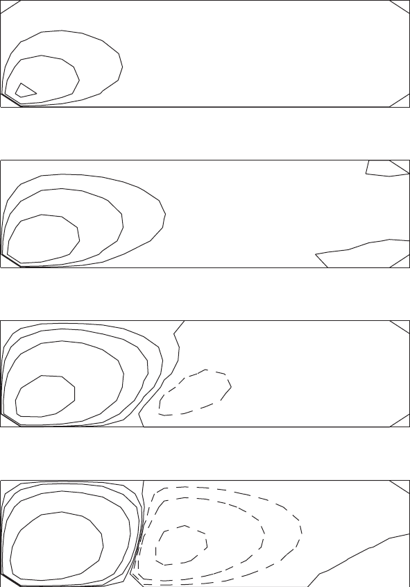
B
´
ENARD AND TAYLOR INSTABILITIES 241
T = 0.025
T = 0.05
T = 0.125
T = 0.2
Time Series for Program 4.2.
counterclockwise motion starts to appear at the center of the bottom plate, as
shown at T = 0.2. The plots for T = 0.25, 0.5, and 0.75 describe the expansion
of this bubble and the continuing intensification of the motion in all three cells.
At T = 1.0, when
NSTEP = 400, the sizes of all three cells are approximately
equal. Printed numerical data disclose that at this instant the strongest motion