Biringen S., Chow C.-Y. An Introduction to Computational Fluid Mechanics by Example
Подождите немного. Документ загружается.

242 NUMERICAL SOLUTION OF THE INCOMPRESSIBLE NAVIER-STOKES EQUATION
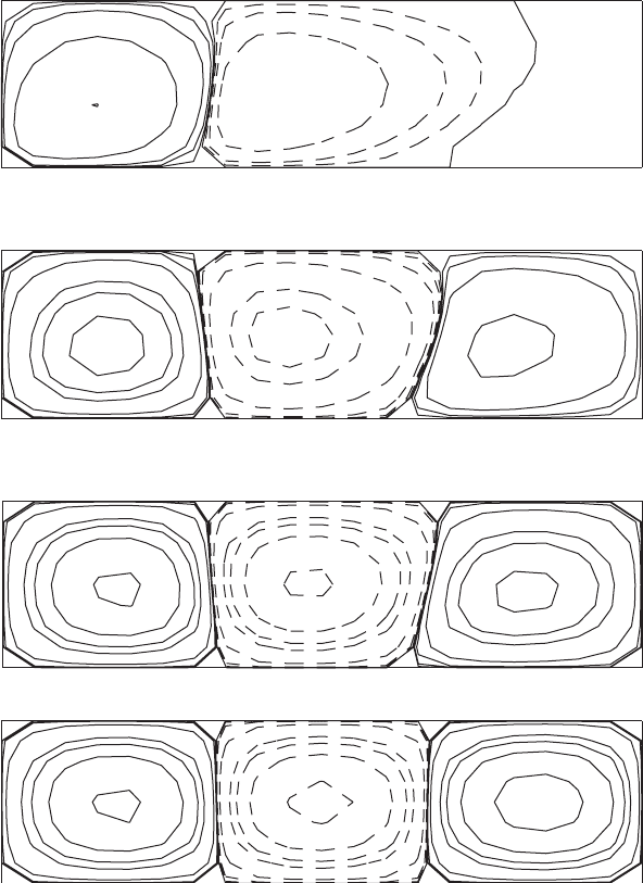
T = 0.25
T = 0.5
T = 0.75
T = 1
Time Series for Program 4.2. (continued)
occurs in the cell on the right, and the cell on the left is the weakest. This
situation is not always true, however. Subsequent data show that as time increases,
the motion in the left cell is strengthened, whereas those in the other two are
weakened. At T = 5.0 the cell on the left becomes the strongest and the middle
one the weakest. The differences in peak velocities among the cells are within
20% of the value in the left cell.
B
´
ENARD AND TAYLOR INSTABILITIES 243
After T = 1.0 the changes in stream pattern are not drastic. At T = 5.0the
left boundary of the middle cell has shifted to the right from its position shown
in the plot for T = 1.0. The displacement of the lower portion of that boundary
is a little longer than that of the upper portion, resulting in a curved interface.
Although a steady state has not been reached yet at T = 5.0, the flow does not
seem to have any further significant changes.
Temperature profiles are not plotted in the output because of their slow varia-
tion with respect to time. In general, the isothermal lines, except those for θ = 0
and 1, have the shape of the cutaway view of an opened umbrella.
Since the pictures shown in the output describe only the behavior of half of
the flow, the total number of convective cells to appear in the channel under the
present arrangement is two at the beginning, changes to four later, and finally
becomes six as the flow continuously evolves. Thus, we start from an unstable
situation of the fluid system having a density inversion; the numerical solution of
the governing equations leads us to a final state, at which the system may be said
to be most stable under the imposed temperature boundary conditions. Once the
computer program has been written, we can easily change the dimensions of the
channel, try different fluid media by varying the Prandtl number, or examine the
effect of temperature gradient by assigning various values to the Grashof number,
and we observe the results of our numerical experiments on the computer.
There are many advantages to using numerical methods to examine the stability
of a fluid flow. If a linearized analytic method, as in Section 3.8, were used to
study the problem considered in this section, a certain number of cells might be
predicted for the onset of instability. However, this prediction may not be valid
at later stages, when the ignored inertial force becomes important, as revealed
by our numerical result that the number of cells is changing with time. It seems
there is no guarantee that the most unstable condition predicted by a linearized
theory will show up in the final state. Furthermore, the inequality in cell size and
the curved cell boundaries are all nonlinear phenomena and cannot be predicted
using linearized theories. Higher-order analyses are generally tedious and are
usually formulated based on the linearized result. The validity of the result so
obtained is also uncertain.
The numerical solution in Program 4.2 is obtained under the assumption of
a two-dimensional flow. The result is unrealistic by virtue of the fact that the
observed convection cells are hexagonal when looking from the top, so that the
actual fluid motion is three dimensional.
Project for Further Study: Perform a numerical experiment on the fluid sys-
tem shown in Fig. 4.3.1, but with some of the boundary conditions changed. It
is now assumed that at the initial instant, θ = 0 everywhere, except θ = 1on
the upper surface. Thereafter, the temperatures at all bounding surfaces will be
kept at their initial values. The upper surface is considered to be a rigid free
surface where both vorticity and shear stress vanish. Assume that there is no ini-
tial motion in the water layer. The situation stated in this problem is somewhat

244 NUMERICAL SOLUTION OF THE INCOMPRESSIBLE NAVIER-STOKES EQUATION
similar to that in an ocean region bounded by two large icebergs, when the upper
surface is heated by the sun.
Project for Further Study: The general circulation of the earth’s atmosphere
is the result of temperature gradients parallel to the earth’s surface caused by
differential solar heating between polar and equatorial regions, even if the ver-
tical stratification of the atmosphere is considered stable. The global horizontal
temperature gradients may cause convective motions in the core of the earth as
well as in the ocean. To study the effect of a horizontal temperature gradient, we
consider a two-dimensional flow contained between two infinitely long parallel
plates whose surfaces are normal to the direction of the gravitational accelera-
tion. Using the distance H between plates as the reference length and introducing
dimensionless variables defined in (4.3.5), we obtain the same set of governing
equations as shown in (4.3.6) to (4.3.10).
For the initial condition we assume that θ = 0 everywhere except that on the
upper plate a periodic temperature distribution
θ = 1 +0.5sin
2π
X
λ
is imposed and is kept unchanged thereafter. The temperature on the bottom plate
is also maintained always at θ = 0.
Because the fluid motion driven by this periodic temperature gradient is also
periodical, we only need to consider the region 0 ≤ X ≤ λ. Periodic boundary
conditions are applied at these two ends. More specifically, if these two vertical
surfaces are represented in index notation by i = 1andm, respectively, and if
we let S be any scalar variable, the periodic condition for S requires that
S
1, j
= S
m, j
S
0, j
= S
m−1, j
S
2, j
= S
m+1, j
Thus, in computing the vertical velocities on the left surface by a central-
differencing scheme, for example, we write
V
1, j
=−
1
2h
(
2,j
−
0,j
)
=−
1
2h
(
2,j
−
m−1,j
)
so that it can be evaluated from the stream function within the concerned fluid
domain. For numerical computation let Pr = 6.75, Gr = 1000, and λ = 2.5. Plot
flow pattern and isothermal contours at several representative time steps.
A flow may become unstable when going along a curved path. This phe-
nomenon can be observed, for example, in the fluid contained between two
B
´
ENARD AND TAYLOR INSTABILITIES 245
concentric cylinders rotating at different speeds. When the two speeds are in
a right combination, the flow cannot maintain its purely angular motion and
becomes unstable, The instability, shown in the form of a series of donut-shaped
ring vortices, was first examined by Taylor (1923) using a linearized analysis
and is usually referred to as the Taylor instability. It turns out that the governing
equations and therefore the analysis for this problem are very similar to those
for the B
´
enard problem just considered.
For such problems, governed by the equations for an incompressible fluid, we
let r
i
and ω
i
be the radius and angular speed of the inner cylinder and r
0
and
ω
0
those of the outer. By choosing ω
−1
i
as the reference time, r
i
as the reference
length, and r
i
ω
i
as the reference speed, a set of dimensionless variables can be
defined, in which is the nondimensional form of the θ-component of vorticity,
whose magnitude is ζ :
R =
r
r
i
, Z =
z
r
i
, U =
u
z
r
i
ω
i
, V =
u
r
r
i
ω
i
T =
t
ω
−1
i
, =
ψ
r
2
i
(r
i
ω
i
)
, =
−ζ
(r
i
ω
i
)/r
i
(4.3.34)
In addition, because of the presence of the angular velocity u
θ
, a new variable is
defined as
W =
ru
θ
r
2
i
ω
i
(4.3.35)
which is the angular momentum expressed in dimensionless form. If the motion
is still assumed to be axisymmetric, the system of nondimensionalized governing
equations consists of
U =
1
R
∂
∂R
(4.3.36)
V =−
1
R
∂
∂Z
(4.3.37)
∂
2
∂R
2
−
1
R
∂
∂R
+
∂
2
∂Z
2
= R (4.3.38)
∂
∂T
=−
∂(U )
∂Z
−
∂(V )
∂R
−2
W
R
3
∂W
∂Z
+
1
Re
∂
2
∂R
2
+
1
R
∂
∂R
−
1
R
2
+
∂
2
∂Z
2
(4.3.39)
∂W
∂T
=−
∂(UW )
∂Z
−
∂(VW )
∂R
−
VW
R
+
1
Re
∂
2
∂R
2
−
1
R
∂
∂R
+
∂
2
∂Z
2
W
(4.3.40)
in which Re = r
2
i
ω
i
/ν is the characteristic Reynolds number, and (4.3.40) is the θ
component of the Navier-Stokes equation. The nonlinear tems in these equations
are expressed purposely in the same form.

246 NUMERICAL SOLUTION OF THE INCOMPRESSIBLE NAVIER-STOKES EQUATION
A computational procedure can be set up for solving the rotating flow problem
that is analogous to that used for solving the convection problem. You are then
ready to make numerical studies of the stability and other nonlinear features of
rotating flows through the following suggested problems.
Project for Further Study: Consider an already established steady flow
between infinitely long concentric cylinders, whose boundary conditions are
W = 1atR = 1 (4.3.41)
W =
r
2
0
ω
0
r
2
i
ω
i
at R =
r
0
r
i
(4.3.42)
Since there is no motion in the meridian plane, U = V = 0, so the angular motion
is described by
W =
(A
2
B −1)R
2
+A
2
(1 −B)
(A
2
−1) (4.3.43)
which is the steady-state solution of (4.3.40) satisfying boundary conditions
(4.3.41) and (4.3.42). The parameters
A =
r
0
r
i
and B =
ω
0
ω
i
(4.3.44)
are, respectively, the ratio of the radii and that of the angular speeds; they are
given constants.
The purely angular flow is then perturbed slightly in the meridian plane at
time T = 0. The small perturbation is represented by a weak periodic vorticity
distribution
= 0.01 sin
2π
Z
λ
(4.3.45)
where λ is the dimensionless wavelength. The meridian motion associated with
this vorticity is computed from (4.3.36) and (4.3.37) after the stream function
has been obtained by solving the equation (4.3.38). Consequently, the angular
motion will be modified according to (4.3.40), causing to change. The time
history of the flow variation is then traced by progressing in T .
On solid walls both U and V vanish for all times. Responding to a periodic
disturbance, the resultant fluid motion is also periodic, so that only an axial length
of λ is needed in the computation. The periodic boundary conditions stated in
the Project for Further Study on page 244 are applied at the ends of this fluid
region.
For numerical computation we assume that A = 2, B = 0 (for a stationary outer
cylinder), λ = 4, and Re = 1000. Suggested intervals are h = 0.125 and T =
0.02. The result should show the development of Taylor ring vortices between
the cylinders. Similar flow patterns can be found in the work by Strawbridge and
Hooper (1968), obtained using a slightly different numerical scheme.
B
´
ENARD AND TAYLOR INSTABILITIES 247
2.5 r
0
0.2 r
0
r
0
u
0
ω
0
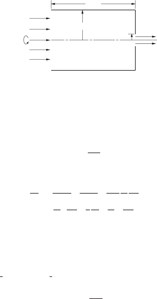
FIGURE 4.3.2 Rotating tube flow through a constriction.
Project for Further Study: Find the steady-state solution for a flow through a
rotating tube having an abrupt contraction, as shown in Fig. 4.3.2. At the entrance
the flow is in rigid body rotation with the same angular speed ω
0
as that of the
tube, and the axial motion is uniform of speed u
0
.
In this problem it is natural to choose the tube radius r
0
as the reference length
and u
0
the reference speed. The dimensionless variables are defined similar to
(4.3.34). Instead of (4.3.35), the dimensionless angular momentum is redefined as
W =
ru
θ
r
2
0
ω
0
(4.3.46)
After they are nondimensionalized, the governing equations are the same as those
for the previous problem, except that (4.3.39) is now replaced by
∂
∂T
=−
∂(U )
∂Z
−
∂(V )
∂R
−
1
2Ro
2
W
R
3
∂W
∂Z
+
1
Re
∂
2
∂R
2
+
1
R
∂
∂R
−
1
R
2
+
∂
2
∂Z
2
(4.3.47)
in which Re = u
0
r
0
/ν is the Reynolds number and Ro = u
0
/2r
0
ω
0
is the Rossby
number, whose value indicates the relative magnitude between the axial and
angular motions of the flow.
Boundary conditions at the entrance have already been specified. For the
remaining boundaries we assume no-slip conditions on the rotating tube wall,
and we require that V = 0 at the exit. Those boundary conditions concerning
stream function are specifically stated as follows: = 0 along the tube axis,
=
1
2
on the wall, =
1
2
R
2
at the entrance and, finally, ∂/∂Z = 0 at the exit.
Note that the velocity along the tube axis is calculated from
U
i,1
=
2ψ
i,2
h
2
(4.3.48)
For a fixed value Re = 50, plot the flow pattern in the meridian plane for
Ro = 2, 1, 0.5, and 0.2.
248 NUMERICAL SOLUTION OF THE INCOMPRESSIBLE NAVIER-STOKES EQUATION
According to a computation (Yih, 1965, p. 260) for an inviscid rotating flow
into a sink (which can be formed by letting the cross-sectional area of our exit
approach zero), at small Rossby numbers the flow is found to separate from the
axis, forming a secondary flow upstream from the sink.
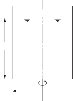
Project for Further Study: In the book by Scorer (1958), the author used a
cartoon as the last problem for discussion. It shows a woman having arrived at
the bottom of a long helical stairway with a tray, serving coffee to two gentlemen.
The caption states: “You’ll find it’s already stirred.” Let us check on the computer
to see if what was said by the woman is correct. An idealized coffee cup is shown
in Fig. 4.3.3. The motion of the cup can be decomposed into a translation and
a rotation. Only the rotation has an effect on the fluid motion inside the cup. At
the initial instant when the woman starts to come down the stairway, there is
no motion in the coffee, and the cup is suddenly given an angular velocity ω
0
.
Suppose the woman is moving at a constant pace so that the angular velocity is
maintained at the same value. The upper surface of the liquid is assumed to be
horizontal and free of shear stresses.
In this problem there is no net axial flow, the dimensionless governing
equations are exactly the same as (4.3.41)–(4.3.45), except that the reference
length and speed are now r
0
and r
0
ω
0
, respectively, and the dimensionless
angular momentum is redefined as W = ru
θ
/r
2
0
ω
0
. We assume r
0
= 0.04 m
and ω
0
= 0.1 π rad/s (computed for 3 revolutions/min). In spite of lacking data
on the physical properties of hot coffee, we use the value of 10
−6
m
2
/s for
kinematic viscosity, which is approximately that of water. The characteristic
Reynolds number, r
2
0
ω
0
/ν, is 500 after rounded off.
Derive two expressions for T, in a form similar to that of (4.3.33), by apply-
ing the quasilinear analysis of Lax and Richtmyer on the governing equations
(4.3.47) and (4.3.40). In your program, at every time step the lowest value of
2r
0
Free Surface
r
0
ω
0
FIGURE 4.3.3 Spin-up in a coffee cup.
PRIMITIVE VARIABLE FORMULATION: ALGORITHMIC CONSIDERATIONS 249
T , which is obtained by searching through the values at all grid points, is
to be used for numerical computations. Selectively plot the flow pattern until
the dimensionless time reaches the value 8. The reference time in this problem
is 1/ω
0
.
This is a simplified spin-up problem, studying the secondary flows and the
development of boundary layers on surfaces in a rotating fluid. The spin-up
problems that interest geophysicists and astrophysicists are usually concerned
with more complex geometries and may include other effects, such as buoyancy
and electromagnetic forces. A general description of the spin neg up phenomenon
can be found in Greenspan (1968).
4.4 PRIMITIVE VARIABLE FORMULATION: ALGORITHMIC
CONSIDERATIONS
We consider the numerical solution of the two-dimensional, incompressible, time-
dependent Navier-Stokes equation written in primitive variable form, where the
unknowns are the two velocity components and the pressure. As we have seen in
Chapter 3, the governing equations, i.e., the (scalar) continuity equation (3.1.6)
and the (vector) equation of motion (3.1.7) are obtained from mass conservation
and momentum conservation laws. We also recall that in incompressible flows
density is constant, and the energy equation is important only when there is
surface heating as in the Benard problem. It was also shown in Chapter 3 that
as opposed to the primitive variables, in the vorticity-stream function formula-
tion of the governing equations, the pressure gradient term does not explicitly
appear. In this section, we will first reexamine several second-order accurate finite
difference formulas that have been widely used for the solution of incompress-
ible flow problems in primitive variable form. We will then introduce efficient
numerical algorithms for the solution of tridiagonal systems of linear equations
that result from implicit time advancement of the viscous terms. The solution for
pressure, staggered mesh arrangements, time advancement will be introduced in
Section 4.5, where we also consider a canonical model problem consisting of the
flow in a lid-driven square cavity.
Generally, finite difference formulas with second-order accuracy in space and
first-order in time are sufficiently accurate for a large number of problems, espe-
cially when the transients in the solution are not of particular interest. However,
there are situations where the time dependency of the solution is important,
such as in turbulent and transitional flows. Also, if the flow has a rapid mean
transient, time accuracy will be of interest. We will explore two popular and
efficient methods that are second-order accurate in both time and space that have
been used frequently for the computation of time-dependent, low-speed, incom-
pressible flows. To introduce these methods, we will first consider the model
convection (hyperbolic) and the model diffusion (parabolic) equations. Subse-
quently, we will apply these methods to the numerical integration of the primitive
variable form of the governing equations.
250 NUMERICAL SOLUTION OF THE INCOMPRESSIBLE NAVIER-STOKES EQUATION
From (2.13.8), the one-dimensional nonlinear convection equation is written as
∂u
∂t
+u
∂u
∂x
= 0 (4.4.1)
where u is the velocity, t is time, and x is the spatial coordinate. Let us use Taylor
series expansion around the grid point (i, n) with respect to the coordinates (x, t),
with u
t
= ∂u/∂t, u
tt
= ∂
2
u/∂t
2
:
u
n+1
i
= u
n
i
+(u
t
)
n
i
t +(u
tt
)
n
i
t
2
2
+O(t
3
) (4.4.2)
As in Section 2.13, the superscript n will denote the time level and the subscripts
i, j are the spatial indices representing coordinates x and y, respectively; the
x increment will be denoted x,they increment y, and the time step as t.
Using one-sided differences,
(u
tt
)
n
i
=
(u
t
)
n
i
−(u
t
)
n−1
i
t
+O(t) (4.4.3)
and substituting (4.4.3) into (4.4.2), we obtain
u
n+1
i
= u
n
i
+(u
t
)
n
i
t +
1
2
(u
t
)
n
i
t −(u
t
)
n−1
i
t
+O(t)t
2
(4.4.4)
and after dividing by t
u
n+1
i
−u
n
i
t
=
3
2
∂u
∂t
n
i
−
1
2
∂u
∂t
n−1
i
+O(t
2
) (4.4.5)
Now, from (4.4.1) let us define
∂u
∂t
=−u
∂u
∂x
≡ H (4.4.6)
Substituting into (4.4.5), we obtain
u
n+1
i
−u
n
i
t
=
3
2
H
n
i
−
1
2
H
n−1
i
+O(t
2
) (4.4.7)
Equation (4.4.7) is called the Adams-Bashforth method, and with second-order
central differences in space, the spatial accuracy of this scheme becomes O(x
2
).
Linear stability analysis indicates that this method is mildly but unconditionally
unstable, and the amplification factor can be written as
λ = 1 +O(t
2
) (4.4.8)

PRIMITIVE VARIABLE FORMULATION: ALGORITHMIC CONSIDERATIONS 251
In long-term time-accurate calculations, this instability remains bounded if the
time step is subject to the Courant number restriction, i.e.,
C ≡
u
max
t
x
≤ 1 (4.4.9)
As shown in Section 2.10, this condition is obtained from the von Neu-
mann analysis, which assumes the error function to be periodic (nonperiodic
boundary conditions are not taken into account) and the equation to be locally
linear. Therefore, for nonlinear equations such as (4.4.1), it is generally required
to choose t (generally by trial and error) such that C is considerably less
than one. We note that although the convective term is nonlinear (quasi-linear),
(4.4.7) can be solved algebraically because explicit finite difference formulas used
for the nonlinear terms do not result in nonlinear difference equations, whereas
implicit formulas used on the nonlinear convective terms will result in nonlin-
ear difference equations. The solution of such nonlinear difference equations will
necessitate local linearization or iterative improvement, which will increase com-
puter resource requirements (Tannehill, Anderson, and Pletcher, 1997, p. 449).
Generally, the inclusion of a diffusive term improves the stability of the Adams-
Bashforth (AB) method.
We also note that to advance the velocity field to time level (n + 1) using
(4.4.7), we need two levels of initial data, at time level n and at time level
(n −1). This can be accomplished by initially using a one-step method, such as
the Euler explicit method for the first time step, and then using that result and
the given initial conditions as the initial data for the second time step to start
the AB solution process. The Euler explicit method for the convection–diffusion
equation can be written as
u
n+1
i
−u
n
i
t
= H
n
i
+O(t) (4.4.10)
Thus, for the first time step only, the time accuracy of the AB method is first
order.
Let us now consider the one-dimensional nonlinear Burgers equation
(nonlinear convection–diffusion equation), which is a more realistic model for
the Navier-Stokes equation,
∂u
∂t
+u
∂u
∂x
= ν
∂
2
u
∂x
2
(4.4.11)
where ν is some transport coefficient, for example, the kinematic viscosity of
the fluid. Rewriting (4.4.6) as
∂u
∂t
= ν
∂
2
u
∂x
2
−u
∂u
∂x
≡ H (4.4.12)
and using the Adams-Bashforth formula (4.4.7) with central differences in
space, we obtain
u
n+1
i
−u
n
i
t
=
3
2
H
n
i
−
1
2
H
n−1
i
+O(t
2
, x
2
) (4.4.13)