Caers J. Modeling Uncertainty in the Earth Sciences
Подождите немного. Документ загружается.

P1: OTA/XYZ P2: ABC
JWST061-02 JWST061-Caers March 30, 2011 18:55 Printer Name: Yet to Come
2.5 RANDOM VARIABLES 21
2.5 Random Variables
At this point, we have studied two separate issues: (1) how to make numerical summaries
of data, and (2) the study of “probability” in general without considering any data. In
this section we will establish a link between the two – to try to quantify probabilities
or other interesting properties from the data set. A key link will be the concept of the
random variable. A random variable is a variable whose value is a numerical outcome
of a random experiment. A random variable is not a numerical value itself. It can take
various outcomes/values, but we do not know, in advance, exactly which value it will take.
Examples are rolling a dice, drawing a card from a deck, sampling a diamond stone from
a diamond deposit. All of these are variables that can be described by a random variable.
We will use as a capital letter such as X or Y to denote a random variable. The capital
letter is important, because we use it to indicate that the value is unknown. The outcome
of a random variable is then denoted by a small letter such as x or y.
P(X ≤ x): denotes the probability that the random variable X is smaller than a given
outcome x. Recall that “X ≤ x” is termed an event.
2.5.1 Discrete Random Variables
A random variable that can take only a limited set of outcomes or values is termed a dis-
crete random variable. An example is rolling a dice: there are only six possible outcomes.
The frequency at which the outcomes occur or the way the random variable is distributed
can be described by a probability mass function using the following notation:
p
X
(a) = P(X = a)
for dice: P(X = 1) = p
X
(1) = 1/6; P(X = 2) = p
X
(2) = 1/6, and so on. Note the notation
p
X
(a), which means that we evaluate the probability for random variable X to take the
value a.
2.5.2 Continuous Random Variables
While in the discrete case, the frequency of possible outcomes can be counted, the number
of possible outcomes cannot be counted for a continuous random variable. In fact, there
are an infinite number of possibilities. Because of this, P(diamond size = 1 ct) = 0 be-
cause there are an infinite (at least theoretically) possibilities, hence any number divided
by infinite is zero. There are two ways to describe the possible variations of a continuous
random variable. Both ways are equivalent. (1) probability density function (pdf ) and
(2) cumulative distribution function (cdf).
2.5.2.1 Probability Density Function (pdf)
The probability density function, which we denote as f
X
(x), is defined as an integral of a
positive function and this integral (surface area) denotes a probability:
P(a ≤ X ≤ b) =
b
a
f
X
(x)dx
P1: OTA/XYZ P2: ABC
JWST061-02 JWST061-Caers March 30, 2011 18:55 Printer Name: Yet to Come
22 CH 2 REVIEW ON STATISTICAL ANALYSIS AND PROBABILITY THEORY
This seems a very contorted way to define a probability, but we need to do it in this
mathematical way for continuous variables because of the 1/infinite reason mentioned
above. The notation f
X
(x) now also becomes a bit more clear. The function f describing
the probabilistic variation of random variable X is evaluated in the point x.
Some important properties are
+∞
−∞
f
X
(x)dx = 1 “some outcome will occur for sure”
f
X
(x) ≥ 0 “probabilities cannot be negative”
P(X = x) = 0 as discussed above
Does the function value f
X
(x) have any meaning? It certainly does not have the meaning
of a probability. It really only has meaning when comparing two outcomes, x
1
and x
2
.
Then the ratio:
f
X
(x
1
)
f
X
(x
2
)
denotes how many times more (or less) likely the outcome x
1
will occur compared to x
2
.
Note that the term “likely” (also used as likelihood) is not the same as “probability”. For
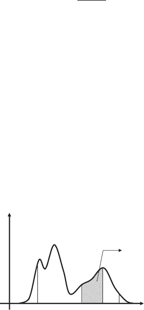
example if the ratio is four, as the case in Figure 2.5, then x
1
is four times more likely to
occur than x
2
. Note that this is not the same as saying “four times more probable.”
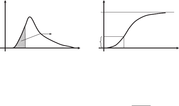
2.5.2.2 Cumulative Distribution Function
A completely equivalent way of describing a random variable is a cumulative distribution
(Figure 2.6):
F
X
(x) = P(X ≤ x)
f
X
(x)
x
ba
x
1
Shaded area
represents a probability
x
2
Figure 2.5 Example of a probability density function.
P1: OTA/XYZ P2: ABC
JWST061-02 JWST061-Caers March 30, 2011 18:55 Printer Name: Yet to Come
2.5 RANDOM VARIABLES 23
f
X
(x )
x
F
X
(x)
always between 0 and 1 and never decreases
x
Area A
Area A
1
Figure 2.6 Definition of a cumulative distribution function.
The relationship between F
X
(x) and f
X
(x) is:
F
X
(x) =
x
−∞
f
X
(y)dy ⇒ f
X
(x) =
dF
X
(x)
dx
2.5.3 Expectation and Variance
2.5.3.1 Expectation
Firstly, consider a discrete random variable X with probability mass function p
X
(x). X has
K possible outcomes, say x
1
, x
2
, x
3
, ..., x
k
:
x
1
:P(X = x
1
) = p
X
(x
1
)
x
2
:P(X = x
2
) = p
X
(x
2
)
x
3
:P(X = x
3
) = p
X
(x
3
), etc.
The expected value, using the notation E[X], is defined as:
E[X] =
K
k=1
x
k
P(X = x
k
)
For example: in rolling a dice we have:
Possible outcomes : x
1
= 1, x
2
= 2, x
3
= 3, x
4
= 4, x
5
= 5, x
6
= 6
E[X] = 1 ×
1
6
+ 2 ×
1
6
+ 3 ×
1
6
+ 4 ×
1
6
+ 5 ×
1
6
+ 6 ×
1
6
=
7
2
Apparently, the expected value of X need not be a value that X could assume. So E[X]
is not the value that one “expects” X to have, but rather E[X] is the average value of X in
a large number of repetitions of the experiment.

P1: OTA/XYZ P2: ABC
JWST061-02 JWST061-Caers March 30, 2011 18:55 Printer Name: Yet to Come
24 CH 2 REVIEW ON STATISTICAL ANALYSIS AND PROBABILITY THEORY
In a very similar manner as for discrete variables, we can define the expected value for
continuous variables:
E[X] =
+∞
−∞
xf
X
(x)dx
Instead of a sum, we now use an integral. If we know f
X
(x), then we can calculate this
integral and find E[X]. For example, if
f
X
(x) =
1
√
2
exp
−
1
2
x −
2
then with some calculus this will result in:
E[X] =
+∞
−∞
x
1
√
2
exp
−
1
2
·
x −
2
= .
2.5.3.2 Population Variance
In a sense, the expected value of a random variable is one way to summarize the distri-
bution function of that variable. So how do we summarize the spread of that population?
Equivalently, as we did for the data (where we used the empirical standard deviation), we
also use a measure – the population variance:
Var [ X ] = E
(
X − E
[
X
]
)
2
=
+∞
−∞
(
x −
)
2
f
X
(
x
)
dx
If we use the same function above, then:
Var
[
X
]
=
+∞
−∞
(
x −
)
2
1
√
2
exp
−
1
2
x −
2
dx =
2
2.5.4 Examples of Distribution Functions
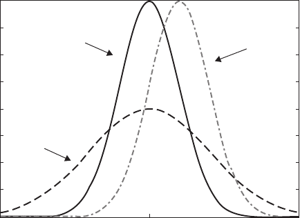
2.5.4.1 The Gaussian (Normal) Random Variable and Distribution
The Gaussian or Normal distribution is a very specific distribution that has the following
mathematical expression:
f
X
(x) =
1
√
2
exp
−
1
2
x −
2
with = population mean or expected value; = population standard deviation. Fig-
ure 2.7 shows some examples with various values for and .
P1: OTA/XYZ P2: ABC
JWST061-02 JWST061-Caers March 30, 2011 18:55 Printer Name: Yet to Come
2.5 RANDOM VARIABLES 25
0.4
μ=0,σ=1
μ=0,σ=2
μ=1,σ=1
0.35
0.3
f
x
0.25
0.2
0.15
0.1
0.05
0
–5 0 5
Figure 2.7 Gaussian distribution for various values of μ and σ .
The Gaussian distribution has two parameters and that can be freely chosen (re-
membering that > 0!). The parameter “regulates” the center of the distribution. It is
the mean if you have an infinite amount of samples from a random variable X with this
distribution. The parameter “regulates” the width of the bell-shaped curve.
Other properties of this distribution function are:
r
population mean = population median
r
population mode = population mean
r
There is no mathematical expression for F
X
(x). You need to use a computer or a table
from a book.
2.5.4.2 Bernoulli Random Variable
The simplest case of a discrete random variable is one that has two possible outcomes.
For simplicity, we will call these categories 0/1.
X = 0 If a trial results in “failure”
X = 1 If a trial results in “success”
A trial should be treated in the broadest sense possible.
Examples:
Finding a diamond larger than 2 ct means “success.”
Rolling ones twice in a row means “success.”
Finding a diamond smaller than 4 ct means “success.”
P1: OTA/XYZ P2: ABC
JWST061-02 JWST061-Caers March 30, 2011 18:55 Printer Name: Yet to Come
26 CH 2 REVIEW ON STATISTICAL ANALYSIS AND PROBABILITY THEORY
In statistics, we call such a random variable a Bernoulli random variable. In geostatis-
tics, we often call it an indicator random variable. The probability distribution is com-
pletely quantified by knowing the probability p of success:
p = P(X = 1) and P(X = 0) = 1 − p
E[X] = 1 × p + 0 × (1 − p) = p
Var [ X ] = (1 − p)
2
p + (0 − p)
2
(1 − p) = p(1 − p)
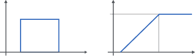
2.5.4.3 Uniform Random Variable
A random variable X is termed uniform when each of its outcomes is equally likely to
occur between any two values a and b, with a < b (Figure 2.8), the probability den-
sity equals:
f
X
(x) =
1
(b − a)
if a ≤ x ≤ b
0 elsewhere
The uniform random variable is important in the context of generating random num-
bers on a computer.
2.5.4.4 A Poisson Random Variable
Examples for which a Poisson random variable is appropriate:
r
The number of misprints on a page of a book
r
The number of people in a community that are 100 years old
r
The number of transistors that fail in their first day of use.
Poisson random variables typically have the following characteristics:
p = probability of the event occurring is small
n = number of trials is large
1
f
X
(x) F
X
(x)
bab
a
xx
Figure 2.8 Uniform pdf and cdf.

P1: OTA/XYZ P2: ABC
JWST061-02 JWST061-Caers March 30, 2011 18:55 Printer Name: Yet to Come
2.5 RANDOM VARIABLES 27
Figure 2.9 Random distribution of points over an area.
In the Earth sciences, the Poisson distribution is important because it has a spatial con-
nection. Take an area with certain objects (diamonds, trees, plants, earthquakes). Take a
small box and put it inside this area, as done in Figure 2.9. The random variable describ-
ing the number of points that you will find in the box is a Poisson random variable and
follows the following equation:
p
X
(i) = P(X = i) = e
−
i
i!
= average number of points in the box
In Chapter 5, we will discuss Boolean or object models, where we will simulate ob-
jects in space. To do so we will make use of the Poisson process, that is, the process of
spreading objects randomly in space as done in Figure 2.9. Note that the coordinate X
and Y of each point are also random variables, namely uniform random variables.
2.5.4.5 The Lognormal Distribution
A variable X is lognormally distributed if and only if log X is normally/Gaussian dis-
tributed. So, if we calculate the log of the data, then the histogram should look like a
normal distribution in case that variable is lognormally distributed. The lognormal dis-
tribution has, therefore, two parameters – mean and variance. The lognormal distribution
can be extremely skewed. Hence, it is an ideal candidate for describing skewed data sets.
The lognormal variable is also positive. This makes it a very useful distribution for most
Earth Science data which are strictly positive; permeability (Darcy), magnitudes, and
grain sizes (mm), for example, are often lognormal.
P1: OTA/XYZ P2: ABC
JWST061-02 JWST061-Caers March 30, 2011 18:55 Printer Name: Yet to Come
28 CH 2 REVIEW ON STATISTICAL ANALYSIS AND PROBABILITY THEORY
2.5.5 The Empirical Distribution Function versus
the Distribution Model
A random variable X describes the entire population of possible outcomes, and its distri-
bution (pdf or cdf) describes in detail which of these outcomes are more likely to occur
than others. F
X
(x)orf
X
(x) are also termed the distribution model of the population. Un-
fortunately, we do not know the entire population, and we certainly do not know F
X
(x)
or f
X
(x). We only have data, that is, a set of values or outcomes of sampling. Using the
data, we will have to guess what f
X
(x) and F
X
(x) are. To do this, we will use the empirical
distribution function, which is essentially the “distribution model of the data” and not the
entire population of X. Just as for the population, we have an empirical pdf and cdf.
Empirical pdf =
ˆ
f
X
(x) = density distribution obtained from the data. The histogram
is, in fact, a graphical representation of the empirical pdf, so we will call
ˆ
f
X
(x) the
histogram.
Empirical cdf =
ˆ
F
X
(x) = the cumulative distribution function based upon the data. It
is constructed as shown in Figure 2.10.
r
Sort the data and plot them on the x-axis.
r
A cumulative probability specifies the probability of being below a threshold, so for the
empirical cdf this becomes:
ˆ
F
X
(x) = P(X ≤ observed datum x)
P(X ≤ x
1
) = 1/6 then 16% of the data is less than or equal to x
1
= 3.2.
P(X ≤ x
2
) = 2/6 then 33% of the data is less than or equal to x
2
= 8.6.
n = 6 data: 10.1 / 15.4 / 8.6 / 9.5 / 20.6 / 3.2
x
20.63.2
10.18.6
9.5 15.4
1
1/6
ˆ
F
x
(x)
Figure 2.10 Empirical cdf.
P1: OTA/XYZ P2: ABC
JWST061-02 JWST061-Caers March 30, 2011 18:55 Printer Name: Yet to Come
2.5 RANDOM VARIABLES 29
2.5.6 Constructing a Distribution Function from Data
An important task in statistical analysis is to figure out which distribution is suitable to
model the data: is it normal? Lognormal? Uniform? Unfortunately, no set of distribution
models exists that is “flexible” enough to fit all the data sets that are observed in nature.
Many of the theoretical distribution models (such the normal and lognormal) stem from
an era where computers were not available and modelers used functions that had only a
few parameters they could easily estimate. In this book, a more computer-oriented method
of interpolation/extrapolation that uses the data themselves to construct a distribution
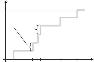
model is advocated. Our anchor point will be the empirical distribution.
Figure 2.11 provides an example, where we assume the data is bounded between 0 and
100. Recall that in the empirical cumulative distribution, we list the data x
1
, ...,x
6
, and
Linear inter/extrapolaon
20.63.2
10.18.6
9.5
15.4
1
100
ˆ
F
20.6
3.2
10.18.6
9.5
15.4
1
100
ˆ
F
1/7
1/(n+1) to allow extrapolaon
6 data samples: 3.2 / 8.6 / 9.5 / 10.1 / 15.4 / 20.6
Figure 2.11 Empirical cdf for building a distribution model directly from data.
P1: OTA/XYZ P2: ABC
JWST061-02 JWST061-Caers March 30, 2011 18:55 Printer Name: Yet to Come
30 CH 2 REVIEW ON STATISTICAL ANALYSIS AND PROBABILITY THEORY
then we make steps of 1/n between them. However, when we want a distribution model
for the entire population, we need to perform two additional steps:
r
Interpolate: We need to know what happens between x
2
and x
3
,orx
3
and x
4
and so on.
r
Extrapolate: We need to know what happens for observations larger than x
6
and
smaller than x
1
. Indeed, the data are only a limited sample of the entire population.
In the entire population it can be expected that some values are large than x
6
and some
are smaller than x
1
.
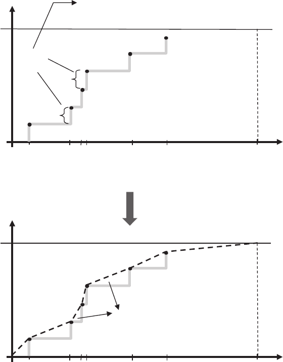
Therefore, we “complete” the empirical distribution by introducing so-called interpo-
lation and extrapolation models, which can be chosen by the modeler, for example a linear
or parabolic/hyperbolic type function. There is no problem to extrapolate lower than x
1
,
but what about values higher than x
6
? There is apparently no room left, because F
X
(X >
x
6
) = 0. The way to solve this problem is to go in steps of 1/(n + 1) instead of 1/n.In
this case, steps of
1
/
7
instead of
1
/
6
are used as shown in Figure 2.11.
In essence, we “patch” together a distribution model F
X
(x) by piecing together inter-
polation and extrapolation models. The advantage of constructing a distribution function
this way is that all one needs to know is essentially a series of numbers to represent a
distribution function. In the current computer era, we have enough memory space to store
a series of, for example, 100 000 values. With the suitable interpolation and extrapola-
tion models, that series of values and the interpolation/extrapolation models represents a
distribution function.
2.5.7 Monte Carlo Simulation
Monte Carlo is a statistical technique that aims at “mimicking” the process of sampling an
actual phenomenon. Therefore, Monte Carlo simulation is often referred to as “sampling”
or “drawing” from a distribution function. When one is actually sampling (not Monte
Carlo sampling), samples are obtained from the field to figure out what, for example, the
population density distribution f
X
(x) is. In Monte Carlo simulation, one assumes that the
distribution f
X
(x) is known, and uses a computer program to sample from it. To construct
a sample experiment, we somehow need to have access to a “random entity,” since we
want our sampling to be fair, that is, no particular value should occur more as described
by the distribution function. For example: how would we simulate flipping a coin on a
computer, such that the outcomes are close to 50/50 head and tail when a large number of
trials are performed? Unfortunately, no random machine exists (a computer is a machine
and still deterministic) that can render a fully random entity. What is available is a so-
called pseudo-random number generator. A pseudo-random number generator is a piece
of software that renders as output a random number upon demand. Such random number
or value, in statistical terms, is simply the outcome of a uniform [0,1] random variable.
Hence, it is a number that is always between zero and one. These numbers are pseudo-
random numbers, because a pseudo random number generator always has to be started
with what is called a “random seed.” For a given random seed, one will always obtain the