Carranza E. Geochemical anomaly and mineral prospectivity mapping in GIS
Подождите немного. Документ загружается.

284 Chapter 8
epithermal Au deposits situated between 0 and 100 m from NNW-trending
faults/fractures plausibly represent concealed deposits. If so, then merging the first two
classes of distances to NNW-trending faults/fractures (Figs. 8-13B and 8-13C) into one
class (Fig. 8-14) is geologically inappropriate because the contained locations of
epithermal Au deposits plausibly represent different levels of erosion. This is a generic
problem in 2-D modeling of mineral prospectivity.
A negative value of
Unc could also occur in the applications of equations (8.8) to
(8.9) if a class of data of a discrete field (e.g., lithologic units as a prospectivity
recognition criterion of favourable host rocks) coincides with more than 50% of the
locations of mineral deposits of the type sought and if
N(C
ji
) is less than 25% of N(T). In
such a case, it is imperative to re-examine the map of the data of a discrete field in terms
of (a) accuracy of class boundaries (e.g., lithologic contacts), (b) compatibility of its
level of data attribute classification (e.g., rock type versus lithologic formation) and thus
scale to the scale of the mineral prospectivity mapping being performed (Raines et al.,
2007), (c) compatibility of its scale to the scale of map of mineral deposit occurrences
and (d) its relevance to the conceptual model of mineral prospectivity under
consideration. In addition, it also imperative to re-examine (a) accuracy of deposit-type
locations and (b) suitability of the unit cell size used in modeling. Addressing these
issues could, more often than not, overcome the occurrence of a negative value of
Unc in
data-driven estimation of EBFs of classes of data of a discrete field.
The occurrence of a negative value of
Unc highlights not only the limitations of
equations (8.8) and (8.9) for data-driven EBF modeling of mineral prospectivity but also
the general limitations of 2-D modeling of mineral prospectivity. Unfortunately, in 2-D
(as well as in 3-D) modeling of mineral prospectivity, there is no rule-of-thumb for the
correct interval or number of classes into which evidential data of continuous fields must
be discretised. Thus, the occurrence of a negative of
Unc provides the opportunity to re-
examine if the data sets are accurate and if classes of evidential data are sound in the
context of mineral deposit occurrence and the scale of mineral prospectivity mapping
being performed. The caveats of data-driven estimation of EBFs thus provide for a
knowledge-guided data-driven modeling of mineral prospectivity (Carranza et al.,
2008a) and they preclude application of the technique as a ‘black-box’ method in which
the geological significance of the modeling procedures is overlooked. The examples
discussed above demonstrate that performing model calibration experiments with
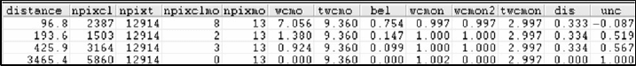
Fig. 8-14. Illustration of occurrence of a negative value for Unc by application of equations (8.8),
(8.9) and (8.10) for data-driven estimation of EBFs of classes of data with respect to deposit-type
locations. The classified data are distances (m) to NNW-trending faults/fractures, which are
considered in predictive modeling of epithermal Au prospectivity in Aroroy district (Philippines).
See text for further explanations and Fig. 8-13C for the names of columns.
Data-Driven Modeling of Mineral Prospectivity 285
different classes of data is imperative in knowledge-guided data-driven creation of
predictor maps (cf. Roy et al., 2006), not only via application of the data-driven EBFs
but also via application of the other data-driven methods listed in Tables 8-I and 8-II.
Nevertheless, the examples discussed above demonstrate that, provided that the classes
of evidential data are prudently examined and properly calibrated, the applications of
equations (8.8) to (8.10) for data-driven estimation of EBFs result in geologically
meaningful empirical spatial associations between deposit-type locations and indicative
geological features and, thus, are useful in the creation of predictor maps for mineral
prospectivity mapping.
Integration of data-driven EBFs
Data-driven estimates of EBFs are calculated and then stored usually in attribute
tables associated with the individual
X
i
spatial evidence maps (Figs. 8-11, 8-13 and 8-
14). Attribute maps of EBFs (i.e., predictor maps) for each of the
X
i
spatial evidence
maps are then created. Only attribute maps of
Bel
i
, Dis
i
and Unc
i
are used for integration
of predictor maps according to the application of Dempster’s (1968) rule of combination.
We recall from the introduction to EBFs in Chapter 7 that, according to Walley (1987),
Dempster’s (1968) rule of combination is generally neither suitable for combining
evidence from independent observations nor appropriate for combining prior beliefs with
observational evidence. This means that Dempster’s (1968) rule of combining EBFs is
suitable in modeling of mineral prospectivity because predictor maps used in most, if not
all, cases are conditionally dependent with respect to locations of mineral deposits of the
type sought for at least two reasons. Firstly, many predictor maps of mineral
prospectivity are derived from a common data set (e.g., maps of proximity to individual
sets of faults/fractures are derived from a geological map), which means that they are to
some extents ‘observationally’ dependent on each other. Secondly, predictor maps each
represent Earth processes that, at some periods in the geologic time scale and at some
environments in the Earth’s crust, interacted simultaneously with each other and caused
the formation of mineral deposits. Inferences about the inter-play of geological processes
involved in mineralisation can be represented in the logical (or sequential) integration of
predictor maps portrayed as EBFs.
The formulae for combining maps of EBFs via either an AND or an OR operation
(An et al., 1994a), according to Dempster’s (1968) rule of combination, are given in
Chapter 7 (equations (7.14)-(7.16) and (7.17)-(7.19)) and are not repeated here. An AND
or an OR operation represents a function
f in equation (8.2). An inference network is
applied to logically combine predictor maps representing EBFs of two sets of spatial
evidence at a time. An inference network is a series of logical steps, each of which
represents a hypothesis of inter-relationship between two sets of processes (portrayed in
predictor maps) that represent (a) controls on the occurrence of a geo-object (e.g.,
mineral deposits) and/or (b) spatial features that indicate the presence of the geo-object.
The inference network applied in the knowledge-driven Boolean logic modeling (see
Chapter 7, Fig. 7-4) and in the knowledge-driven evidential belief modeling (Chapter 7)
286 Chapter 8
is also applied to logically integrate the data-driven estimates EBFs of the spatial
evidence maps of epithermal Au prospectivity in the case study area.
Case study application of data-driven EBFs
The objectives of the case study are to illustrate the utility, in mineral prospectivity
mapping, of (a) coherent deposit-type locations and (b) coherent proxy deposit-type
locations. The spatial evidential data sets used in the case study are given in the
introduction section of this chapter. The strategies applied for cross-validation of the
predictive models, portrayed as integrated values of
Bel, of epithermal Au prospectivity
in the case study area are given the preceding section.
Calibration experiments were performed not only in deriving data-driven estimates of
EBFs for classes of catchment basin analysis anomaly values (Fig. 8-11) and classes of
proximity to NNW-trending faults/fractures (Fig. 8-13) but also in deriving data-driven
estimates of EBFs for classes of proximity to NW-trending faults/fractures and
proximity to intersections of NNW- and NW-trending faults/fractures. These calibration
experiments resulted in common properly calibrated classes of each of the data sets
(Table 8-IV) with respect to the training sets of 13 known and 11 coherent (out of the 13
known) locations of epithermal Au deposits and 86 randomly-selected and 86 coherent
proxy locations of epithermal Au deposits (Fig. 8-8). The data classes in Table 8-IV are
considered properly calibrated because the plots of the data-driven estimates of
Bel
versus the upper limits of the properly calibrated classes with respect to the different
training sets are not noisy (Fig. 8-15) and facilitate recognition of threshold data values
that are associated spatially with the training sets of deposit and proxy deposit locations.
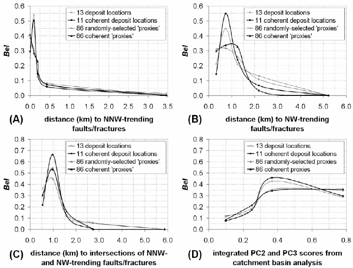
The graphs in Fig. 8-15 indicate that the training deposit and proxy deposit locations are
mostly within 0.3 km of NNW-trending faults/fractures and within 1.5 km of NW-
trending faults/fractures and intersections of NNW- and NW-trending faults/fractures
and that the training deposit and proxy deposit locations coincide mostly with integrated
PC2 and PC3 multi-element scores greater than 0.3. These results are generally
consistent with the results of analyses of spatial associations between the same spatial
data sets and the locations of epithermal Au deposits in the study area (see Chapter 6,
Table 6-IX).
The graphs in Fig. 8-15 show that, for the range of data values that are associated
spatially with the deposit and proxy deposit locations, the applications of the training
sets of coherent deposit and proxy deposit locations result in higher values of
Bel than
the applications of the training sets of all deposit locations and randomly-selected proxy
deposit locations. Conversely, the graphs in Fig. 8-15 show that, for the range of data
values that lack spatial association with the deposit and proxy deposit locations, the
applications of the training sets of all deposit locations and randomly-selected proxy
deposit locations result in higher values of
Bel than the application of the training sets of
coherent deposit and proxy deposit locations. These results imply that, compared to the
applications of all deposit locations and randomly-selected proxy deposit locations, the

Data-Driven Modeling of Mineral Prospectivity 287
applications of coherent deposit and proxy deposit locations result in better predictive
models of epithermal Au prospectivity in the study area.
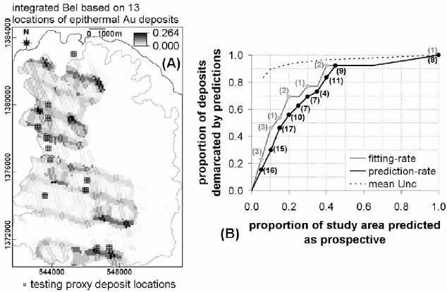
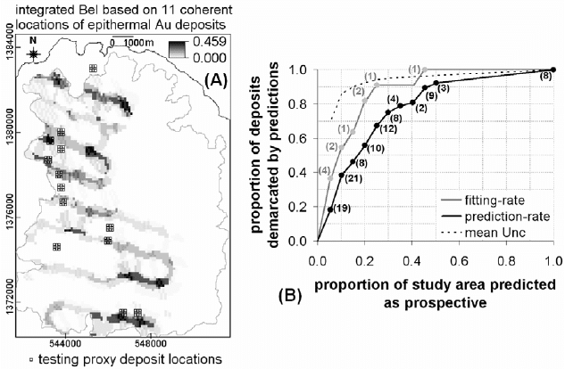
The map of integrated values of
Bel based on the training set of 13 known locations
of epithermal Au deposits (Fig. 8-16A) and the map of integrated values of
Bel based on
the training set of 11 coherent locations of epithermal Au deposits (Fig. 8-17A) both
show circular patterns of intermediate and high values of integrated
Bel reflecting the
spatial evidence of proximity to intersections of NNW- and NW-trending
faults/fractures. The values of integrated
Bel are highest mostly where the circular
patterns intersect with the patterns reflecting the spatial evidence of proximity to NNW-
trending faults/fractures, which are more conspicuous in Fig. 8-16A than in Fig. 8-17A.
The pattern of intermediate and high integrated values of
Bel in both maps (Figs. 8-16A
and 8-17A) seem odd but are consistent with the conceptual model of epithermal Au
mineralisation in dilational or extensional settings as depicted in Fig. 6-16.
The fitting-rates of the map of integrated values
Bel based on the training set of 11
coherent locations of epithermal Au deposits (Fig. 8-17B) are better than the fitting-rates
of the map of integrated values
Bel based on the training set of 13 known locations of
TABLE 8-IV
Properly calibrated classes of spatial data sets for evidential belief modeling of epithermal Au
prospectivity, Aroroy district (Philippines). Ranges of data values in bold are associated spatially
with the epithermal Au deposits in the case study area (see Chapter 6, Table 6-IX). The plots of
values of Bel versus the upper limits of classes of data are shown in Fig. 8-15.
Classes of proximity to NNW
1a
Classes of proximity to NW
2
Class code Range
1b
(km) Class code Range (km)
NNW1
0.00
NW1
0.00 – 0.33
NNW2
0.01 – 0.10
NW2
0.34 – 0.74
NNW3
0.11 – 0.19
NW3
0.75 – 1.26
NNW4
0.20 – 0.43
NW4 1.27 – 2.19
NNW5 0.44 – 3.47 NW5 2.20 – 5.23
Classes of proximity to FI
3
Classes of ANOMALY
4a
Class code Range (km) Class code Range
4b
FI1
0.00 – 0.54
ANOM1
0.369 – 0.781
FI2
0.55 – 0.99
ANOM2
0.252 – 0.368
FI3
1.00 – 1.59
ANOM3 0.100 – 0.251
FI4 1.60 – 2.75 ANOM4
≤0.099
FI5 2.76 – 5.87 ANOM5 ‘no data’
1a
NNW-trending faults/fractures.
1b
Upper limits of proximity range are equivalent to the distances
(m) in the first column of table in Fig. 8-13C.
2
NW-trending faults/fractures.
3
Intersections of
NNW- and NW-trending faults/fractures.
4a
Integrated PC2 and PC3 scores obtained from the
catchment basin analysis of stream sediment geochemical data (see Chapter 5, Fig. 5-12).
4b
Upper
limits of ANOMALY range are the same as values of anomaly in the first column of table in Fig.
8-11C, but in decreasing order.
288 Chapter 8
epithermal Au deposits (Fig. 8-16B). This is why the former map is less ‘noisy’ than the
latter map. The prediction-rates of the map of integrated values of
Bel based on the
training set of 11 coherent locations of epithermal Au deposits (Fig. 8-17B) are also
better than the prediction-rates of the map of integrated values
Bel based on the training
set of 13 known locations of epithermal Au deposits (Fig. 8-16B). For example, if 10%
and 30% of the study area are considered prospective, then the map in Fig. 8-17A has
prediction-rates of 38% and 75% (Fig. 8-17B), respectively, whereas the map in Fig. 8-
16A has prediction-rates of 29% and 70% (Fig. 8-1B), respectively. In addition, the map
of integrated values of
Bel based on the training set of 11 coherent locations of
epithermal Au deposits has lower values of integrated
Unc (Fig. 8-17B) than the map of
integrated values
Bel based on the training set of 13 known locations of epithermal Au
Fig. 8-15. Variations of spatial associations of individual sets of geological features with all and
only coherent locations of epithermal Au deposits and with randomly-selected and coherent proxy
locations of epithermal Au deposits in Aroroy district (Philippines) as depicted by the plots o
f
data-driven estimates of Bel versus upper limits of classes of (A) distances to NNW-trending
faults/fractures, (B) distances to NW-trending faults/fractures, (C) distances to intersections o
f
NNW- and NW-trending faults/fractures and (D) integrated PC2 and PC3 scores obtained from the
catchment basin analysis of stream sediment geochemical data (see Chapter 5, Fig. 5-12).
Data-Driven Modeling of Mineral Prospectivity 289
deposits (Fig. 8-16B). These results illustrate the advantage of using coherent deposit-
type locations in predictive modeling of mineral prospectivity.
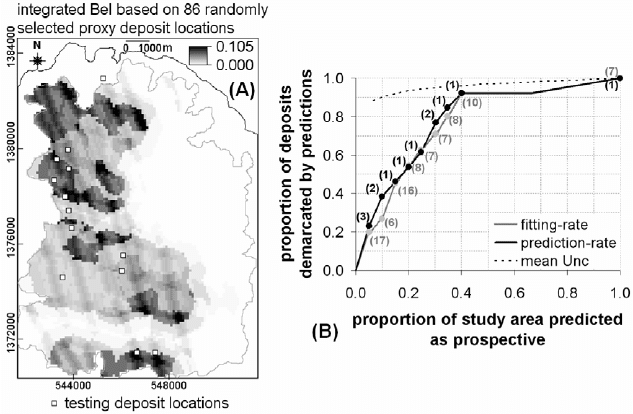
The map of integrated values
Bel based on a training set of 86 randomly-selected
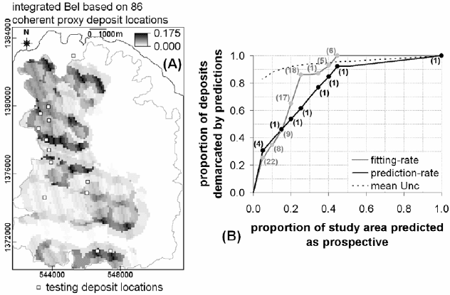
proxy locations of epithermal Au deposits (Fig. 8-18A) and the map of integrated values
Bel based on the training set of 86 coherent proxy locations of epithermal Au deposits
(Fig. 8-19A) also show circular patterns of intermediate and high values of integrated
Bel reflecting the spatial evidence of proximity to intersections of NNW- and NW-
trending faults/fractures. Compared to the former map, the latter map is more similar to
the maps in Fig. 8-16A and 8-17A. The maps in Figs. 8-18A and 8-19A both display
intermediate and high values of integrated
Bel reflecting the patterns of anomalous
sample catchment basins in the western parts of the study area (see Fig. 5-12), although
these patterns are more conspicuous in Fig. 8-18A than in Fig. 8-19A. These
observations indicate that the map of integrated values of
Bel based on the training set of
Fig. 8-16. (A) Epithermal Au prospectivity map of Aroroy district (Philippines) portrayed as
integrated values of Bel of spatial evidence layers with respect to a training set of 13 locations o
f
epithermal Au deposits. Polygon outlined in grey is area of stream sediment sample catchment
basins (see Fig. 4-11). The testing set of 104 proxy deposit locations immediately surrounding
each of the known locations epithermal Au deposits (see Fig. 8-8) is shown as reference to the
prediction-rate. (B) Fitting and prediction-rate curves of, respectively, proportions of training
deposits and testing proxy deposits demarcated by the predictions versus proportion of the study
area predicted as prospective based on the integrated values of Bel. The grey and black dots
represent classes of integrated values of Bel that correspond spatially with certain numbers o
f
training deposit locations (in grey) and certain numbers of testing proxy locations (in black),
respectively.
290 Chapter 8
86 coherent proxy locations of epithermal Au deposits (Fig. 8-19A) portrays patterns
derived from each of the four input predictor maps whilst the map of integrated values
Bel based on a training set of 86 randomly-selected proxy locations of epithermal Au
deposits (Fig. 8-18A) portrays patterns derived mostly from at least two of the four
predictor maps. This is why the fitting-rates of the former map (Fig. 8-19B) are better
than the fitting-rates of the latter map (Fig. 8-18B).
In terms of prediction-rate, the map of integrated values of
Bel based on the training
set of 86 coherent proxy locations of epithermal Au deposits (Fig. 8-19A) and the map of
integrated values of
Bel based on a training set of 86 randomly-selected proxy locations
of epithermal Au deposits (Fig. 8-18A) both delineate the same percentages (38-54%) of
testing deposit locations if 10-20% of the study area is considered prospective (Figs. 8-
18B and 8-19B). The map of integrated values of
Bel based on a training set of 86
randomly-selected proxy locations of epithermal Au deposits (Fig. 8-18A) is better than
the map of integrated values of
Bel based on the training set of 86 coherent proxy
Fig. 8-17. (A) Epithermal Au prospectivity map of Aroroy district (Philippines) portrayed as
integrated values of Bel of spatial evidence layers with respect to a training set of coherent
locations of epithermal Au deposits. Polygon outlined in grey is area of stream sediment sample
catchment basins (see Fig. 4-11). The testing set of 104 proxy deposit locations immediately
surrounding each of the known locations epithermal Au deposits (see Fig. 8-8) is shown as
reference to the prediction-rate. (B) Fitting and prediction-rate curves of, respectively, proportions
of training deposit locations and testing proxy deposit locations demarcated by the predictions
versus proportion of the study area predicted as prospective based on the integrated values of Bel.
The grey and black dots represent classes of integrated values of Bel that correspond spatially with
certain numbers of training deposit locations (in grey) and certain numbers of testing locations (in
black), respectively.
Data-Driven Modeling of Mineral Prospectivity 291
locations of epithermal Au deposits (Fig. 8-19A) if more than 20% of the study area is
considered prospective. However, if 5% of the study area is considered prospective, then
the latter map delineates 31% of the testing deposit locations, whereas the latter map
delineates 23% of the testing deposit locations. Therefore, because mineral prospectivity
mapping aims to constrain the sizes of exploration targets in order to increase the chance
of mineral deposit discovery, then the map of integrated values of
Bel based on the
training set of 86 coherent proxy locations of epithermal Au deposits (Fig. 8-19A) is
better than the map of integrated values of
Bel based on a training set of 86 randomly-
selected proxy locations of epithermal Au deposits (Fig. 8-18A). In addition, the former
map has lower values of integrated
Unc (Fig. 8-19B) than the latter map (Fig. 8-18B).
These results illustrate the advantage of, not just proxy but, coherent proxy deposit-type
locations in predictive modeling of mineral prospectivity. The results also imply the
disadvantage of random selection of training (proxy) deposit-type locations for
predictive modeling of mineral prospectivity.
Fig. 8-18. (A) Epithermal Au prospectivity map of Aroroy district (Philippines) portrayed as
integrated values of Bel of spatial evidence layers with respect to a training set of 86 randomly-
selected (from 104) proxy locations of epithermal Au deposits (Fig. 8-8). Polygon outlined in grey
is area of stream sediment sample catchment basins (see Fig. 4-11). The testing set of locations o
f
13 epithermal Au deposits is shown as reference to the prediction-rate. (B) Fitting and prediction-
rate curves of, respectively, proportions of training proxy deposits and testing deposits demarcated
b
y the predictions versus proportion of the study area predicted as prospective based on the
integrated values of Bel. The grey and black dots represent classes of integrated values of Bel that
correspond spatially with certain numbers of training proxy deposit locations (in grey) and certain
numbers of testing deposit locations (in black), respectively.
292 Chapter 8
The results of the case study demonstrate the usefulness of data-driven evidential
belief modeling of mineral prospectivity. Despite of the caveats of data-driven
estimation of EBFs of classes of individual spatial evidence layers, Dempster’s (1968)
rule of combination provides for calibration experiments in integrating predictor maps in
order to emulate the inter-play of processes involved in mineralisation (see Chapter 6).
Emulating the simultaneous interactions of various processes involved in mineralisation
is the main difficultly in predictive modeling of mineral prospectivity. A way to
overcome this difficulty is to quantify simultaneously the spatial associations of the
predictor variables with the target variables. This is conceivably the reason why there are
more multivariate techniques (Table 8-II) than bivariate techniques (Table 8-I) for
mineral prospectivity mapping. This is not to say, however, that multivariate techniques
are automatically superior to bivariate techniques because many of the latter techniques
do not involve inference systems for combining predictor maps of mineral prospectivity.
Let us now turn to one of these multivariate techniques – discriminant analysis.
Fig. 8-19. (A) Epithermal Au prospectivity map of Aroroy district (Philippines) portrayed as
integrated values of Bel of spatial evidence layers with respect to a training set of 86 coherent
proxy locations of epithermal Au deposits (Fig. 8-8). Polygon outlined in grey is area of stream
sediment sample catchment basins (see Fig. 4-11). The testing set of locations of 13 epithermal Au
deposits is shown as reference to the prediction-rate. (B) Fitting and prediction-rate curves of,
respectively, proportions of training proxy deposits (grey dots) and testing deposits (black dots)
demarcated by the predictions versus proportion of the study area predicted as prospective based
on the integrated values of Bel. The grey and black dots represent classes of integrated values o
f
Bel that correspond spatially with certain numbers of training proxy deposit locations (in grey) and
certain numbers of testing deposit locations (in black), respectively.
Data-Driven Modeling of Mineral Prospectivity 293
DISCRIMINANT ANALYSIS OF MINERAL PROSPECTIVITY
Discriminant analysis (DA) has a long history of application in exploration
geochemistry (e.g., Bull and Mazzucchelli, 1975; Govett et al., 1975; Beauchamp et al.,
1980; Howarth, 1983b; Clarke et al., 1989; Chork and Rousseeuw, 1992; Yusta et al.,
1998; Singer and Kouda, 2001) and mineral prospectivity mapping (see references in
Table 8-II). The common chief objective of the applications of DA to geochemical
anomaly and mineral prospectivity mapping is to classify every location in a study area
into two mutually exclusive groups – prospective (anomalous or mineralised) and non-
prospective (background or barren) – based on a training set of known deposit-type and
non-deposit locations and multiple sets of data of discriminating (i.e.,
predictor/explanatory) variables at these locations.
Exhaustive explanations of DA are not given here, but readers are referred to Davis
(2002, pp. 471-479) for a thorough introduction to DA and to Harris and Pan (1999) and
Pan and Harris (2000, pp.411-414) for explanations of different methods of DA that can
be applied to mineral prospectivity modeling. The treatment of DA here is limited to the
basic principles and application of the two-group DA method, which is also called Fisher
linear DA (Fisher, 1936) and demonstration of a GIS-based technique for representation
of data of predictor/explanatory variables in DA.
Basic principles and assumptions of linear discriminant analysis
In general, the maximum number of discriminant functions that can be derived for
the classification of groups of data is either equal to the number of groups minus one or
equal to the number of predictor variables, whichever is less. In the two-group DA
(hereafter denoted as LDA; L stands for linear), therefore, there is only one discriminant
function, which is a linear combination of the predictor variables with the following
mathematical form:
pDLpDLDLDL
XbXbXbbS ++++= !
22110
(8.11)
where
S
DL
is the discriminant score for case (location) L in group D, X
pDL
is the value of
predictor variable
p (=1,2,…,n) for case (location) L in group D, b
0
is a constant and b
1
,
b
2
and b
p
are function coefficients. A discriminant function is generated from a training
set of
L cases (locations), for which membership in group D (e.g., deposit or non-
deposit) is known. There are two types of function coefficients derived in DA -
standardised function coefficients and unstandardised function coefficients (Tabachnick
and Fidell, 2007). Note that there is no
b
0
among the standardised function coefficients.
On the one hand, the standardised function coefficients are used for assessing the relative
importance of the predictor variables in classifying the target variable (in this case
deposit and non-deposit locations). On the other hand, the unstandardised function
coefficients are the ones used in equation (8.11) in order to derive values of
S
DL
for the
classification of unknown cases (i.e., unvisited locations) with values for the same sets of