Chattaraj P.K. (Ed.) Quantum Trajectories

Подождите немного. Документ загружается.

204 Quantum Trajectories

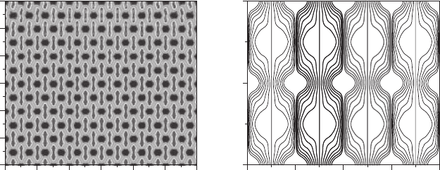
13.2.3 MANY SLITS:THE TALBOT EFFECT AND MULTIMODE CAVITIES

As mentioned above, the number of slits determines the number of domains. Now, as

the number of slits, N , increases, a certain well-organized structure starts to emerge

in the Fresnel region, whose extension also increases. In the limit N →∞, this

structure covers the whole subspace behind the grating and forms a “carpet” with

the particularity that it is periodic along both the direction parallel to the slit grating

(the periodicity is equal to the spacing between the slits or grating period, d) and the

direction perpendicular to the grating, as seen in Figure 13.5a. This is the so-called

Talbot effect [30], very well known in optics. The periodicity (d) along the parallel

direction arises from the presence of well-deﬁned domains with such a periodicity,

which gives rise to a channeling of the quantum ﬂux (as shown in Figure 13.5b in

terms of Bohmian trajectories), similar to having it conﬁned within a waveguide.

This is a physical picture of the well-known Bloch theorem and Born–von Karman

periodic conditions considered when one has periodic lattices in solid state physics,

for example. Along the perpendicular direction, however, we ﬁnd a ﬁrst recurrence at

= d

/λ, known as the Talbot distance (with λ being the wavelength of the incoming

particle beam), which is π-shifted with respect to ρ

(x). Then, a second recurrence

is found at 2z

, which is an exact replica of ρ

(x) (i.e., the wave function that we

have just behind the grating) at 2z

. At other fractional distances of z

, there are

composite, fractional (including fractal-like [46]) replicas of ρ

instead of identical

ones. Talbot carpets can be explained taking into account the periodic conditions

imposed by the grating period and, therefore, can be related to multimode interference

processes [29,30,46]: by generating a superposition with the modes compatible with

such periodic conditions (as is also done with superpositions of the eigenfunctions of

a square box or a harmonic oscillator).

Talbot-like structures are not only observable with slits, but they also appear when

we have periodic surfaces illuminated by a coherent incident beam. In this latter case,

6(a) (b)

z (z

)

z (z

)

–6 –4 –2

x (d)

–2 –1 0

0246

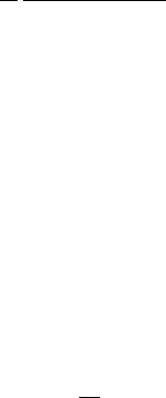
FIGURE 13.5 (a) Talbot carpet arising from the interference of outgoing He-atom beams

with an initial Gaussian proﬁle [30]. (b) Enlargement of the associated Bohmian trajectories,

showing the periodicity of the quantum ﬂux along both x and z.

Quantum Interference from a Hydrodynamical Perspective 205

due to the effect of the attractive and/or repulsive forces mediating the interaction

between the incident beam and the surface, the Talbot pattern will present a certain

distortion near the classical interaction region due to the Beeby effect. This is what

we have called the Talbot–Beeby effect [30].

13.2.4 I

NTERFERENCE IN TWO-DIMENSIONS: VORTICAL DYNAMICS

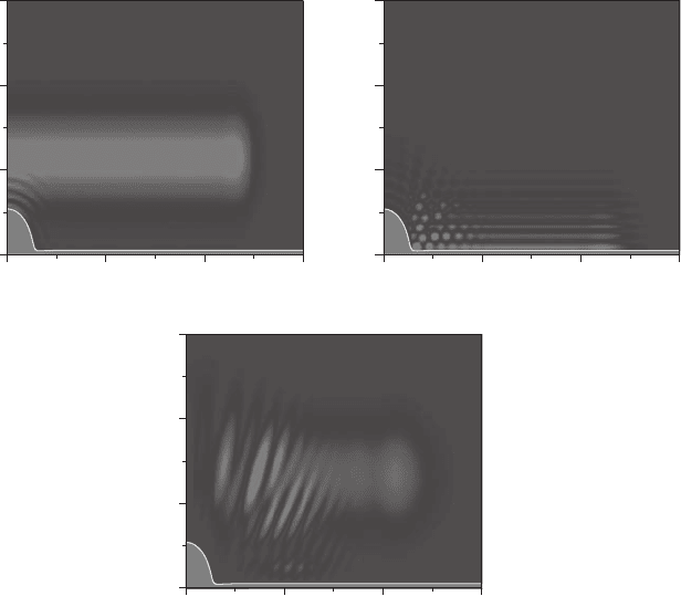
Finally, consider a ﬂat (or almost ﬂat) surface upon which there is an obstacle, such

an adsorbed particle. Due to the presence of the obstacle, an interference-like struc-

ture emerges. The frames shown in Figure 13.6 illustrate the appearance of such a

structure when an incoming quasi-plane wave function (which represents an incident

He-atom beam) approaches an almost ﬂat Pt surface with a CO molecule adsorbed

on it [26, 27]. As a result of the still incoming wave and the outgoing semicircular

wave formed by the adsorbate, a web of vortices appears—far from the adsorbate, the

30(a)

x (a.u.)

40 60

z (a.u.)

30(b)

x (a.u.)

40 60

z (a.u.)

(c)

x (a.u.)

40 60

z (a.u.)

FIGURE 13.6 From (a) to (c), formation of a vortical web when an extended wave function

approaches an imperfection on a surface (adsorbate) [26, 27]. The well-deﬁned vortical web

(b) arises as a consequence of the superposition of the outgoing circular wavefronts and the

(still) incoming wavefront.

206 Quantum Trajectories

(c)

201510

z (a.u.)

x (a.u.)

(a)

201510

z (a.u.)

x (a.u.)

(b)

201510

z (a.u.)

x (a.u.)

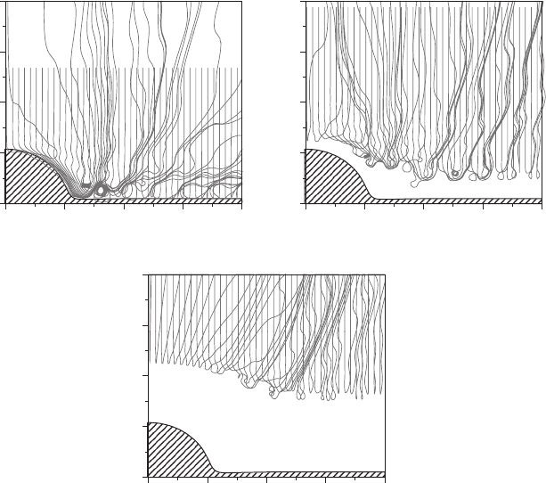
FIGURE 13.7 Quantum trajectories illustrating the dynamics associated with the diffracted

processes represented in Figure 13.6. In each frame, the trajectories have been launched from

the same z

initial position (varying x

), which has been taken at the foremost (a), central

(b) and rearmost (b) positions on the initial wave function.

outgoing wavefront is almost ﬂat and, therefore, we only appreciate the formation of

parallel ripples. By inspecting the associated trajectory dynamics (see Figure 13.7),

we ﬁnd that a vortical dynamics develops around the adsorbate, with quantum tra-

jectories displaying temporary loops around different vortices. Moreover, as in the

case of the soft potential modeling the two slits, here we also ﬁnd that trajectories

started at the regions on the initial wave function further from the adsorbate will not

be able to reach it physically, but will feel a sort of effective potential energy

surface [26–28].

13.3 QUANTUM FLUX ANALYSIS

Consider the coherent superposition described by Equation 13.1, with ψ

and ψ

given by normalized Gaussian wave packets, which propagate initially in opposite,

converging directions and are far enough in order to minimize the (initial) overlap

Quantum Interference from a Hydrodynamical Perspective 207

between them, i.e., ρ

0,1

(r)ρ

0,2

(r) ≈ 0. The dynamics observed will depend on the ratio

between the propagation velocity v

and the spreading velocity v

associated with

the interfering wave functions [44] as well as on their relative weighting factor, α.If

 v

, the interference process is temporary and localized spatially; this collision-

like behavior is typical, for example, of interferometry experiments. On the other hand,

if v

 v

, an interference pattern appears asymptotically and remains stationary

after some time (at the Fraunhofer region); this diffraction-like behavior is the one

observed in slit diffraction experiments, for example.

As can be noticed in Equations 13.5 and 13.8, there are two well-deﬁned contri-

butions related to the effects caused by the exchange of ψ

and ψ

on the particle

motion after interference has taken place. The ﬁrst contribution is even after only

exchanging the modulus or only the phase of the wave packets; the second one

changes its sign with these operations. From the terms that appear in each contri-

bution, it is apparent that the ﬁrst contribution is associated with the evolution of

each individual ﬂux as well as with their combination. Thus, it provides information

about both the asymptotic behavior of the quantum trajectories and also about the

interference process (whenever the condition ρ

(r, t )ρ

(r, t ) ≈ 0 is not satisﬁed).

On the other hand, the second contribution describes interference effects connected

with the asymmetries or differences of the wave packets. Therefore, it will van-

ish at x = 0 when the wave packets are identical although their overlap might be

non-zero.

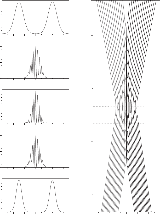
Consider the symmetric collision-like case [44]. From now on, we will refer to

the domains associated with ψ

and ψ

as I and II, respectively. Usually, after the

wave packets have maximally interfered at a given time t

int

max

(see panel for t = 0.3, on

the left, in Figure 13.8), it is commonly assumed that ψ

moves to the domain II and

to I. However, if the process is considered from the viewpoint of quantum ﬂuxes

or Bohmian trajectories (see right-hand-side panel in Figure 13.8), the non-crossing

property forbids such a possibility.As infers from Equation 13.8, for identical, counter-

propagating wave packets the velocity ﬁeld is zero along x = 0 at any time, i.e., there

cannot be any probability density (or particle) ﬂow from domain I to II, or vice versa.

Therefore, after interference (see panels for t>0.3, on the left, in Figure 13.8),

each outgoing wave packet can be somehow connected (through the quantum ﬂux

or, equivalently, the corresponding quantum trajectories) with the initial wave packet

within its domain and the whole process can be understood as a sort of bouncing

effect undergone by the wave packets after reaching maximal interference (maximal

“approaching”).

Although the trajectory bundles do not cross each other, they behave asymptoti-

cally as if they did [44]. From a hydrodynamic viewpoint, this means that the sign of

the associated velocity ﬁeld will change after the collision—before the collision its

sign points inwards (toward x = 0); at t

int

max

it does not point anywhere, but remains

steady; and, after the collision, it points outwards (diverging from x = 0). This

conciliates with the standard description of wave-packet crossing (based on a literal

interpretation of the superposition principle), which can be understood as a “transfer”

of the probability functions describing the ﬂuxes from one domain to the other. That

is, in analogy to classical particle–particle elastic collisions, where particles remain

208 Quantum Trajectories

1.0

0.6

0.5

0.4

0.3

0.2

0.1

0.0

t = 0.6

t = 0.4

t = 0.3

t = 0.25

t = 0

0.5

0.0

1.0

0.5

0.0

1.0

0.5

0.0

1.0

0.5

0.0

1.0

0.5

ρ (x)

t (a.u.)

0.0

–6 –4 –2 2 4 60

x (a.u.)

–6 –4 –2 2 4 60

x (a.u.)

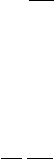
FIGURE 13.8 Left: From bottom to top, the frame sequence shows the appearance of inter-

ference in a collision-like process (v

 v

) through the probability density ρ [44]. Times are

indicated on the top-right corner of each frame. Right: Quantum trajectories illustrating the

probability ﬂow as the two wave packets approach and then separate again after the “collision.”

The horizontal dashed lines denote the intermediate stages shown in the left column.

Quantum Interference from a Hydrodynamical Perspective 209

as such (i.e., the collision does not give rise to the formation of new particles) though

their momentum is exchanged, here the particle swarms exchange their probability

distributions “elastically.” This process can be described as follows. Initially, depend-

ing on the trajectory domain, they can be described approximately by the equations

of motion

≈∇S

/m or

≈∇S

/m. Now, asymptotically (i.e., for t  t

int

max

Equation 13.8 can be expressed as

r ≈

∇S

+ ρ

∇S

+ ρ

, (13.10)

where we have assumed ρ

(x, t )ρ

(x, t ) ≈ 0. Note that this approximation also means

that ρ = ρ

+ ρ

is non-vanishing only on those space regions covered either by ρ

or by ρ

. Speciﬁcally, in domain I, ρ ≈ ρ

, and in II, ρ ≈ ρ

. Inserting this result

into Equation 13.10, we obtain that

≈∇S

/m and

≈∇S

/m, which repro-

duce (and explain) the asymptotic dynamics. This trajectory picture thus provides

us with a totally different interpretation of interference processes: although proba-

bility distributions transfer, particles always remain within the domain where they

started from.

In diffraction-like cases, the spreading is faster than the propagation, this being

the reason why we observe the well-known quantum trajectories of a typical two-slit

experiment in the Fraunhofer region [25,26]. It is relatively simple to show [30] that,

in this case, the asymptotic solutions of Equation 13.8 are

x(t) ≈ 2πn

(

)

, (13.11)

with n = 0, ±1, ±2, .... That is, there are bundles of quantum trajectories whose

slopes are quantized quantities (through n) proportional to v

. This means that, when

Equation 13.8 is integrated exactly, one will observe quantized trajectory bundles

which, on average, are distributed around the value given by Equation 13.11.

13.4 EFFECTIVE INTERFERENCE POTENTIALS

Consider now the problem of a wave packet scattered off an impenetrable potential

wall, with v

[44]. At the time of maximal interference between its still incident

(forward, f ) part and the already outgoing (backward, b) part (see Figure 13.6b, for

example), the corresponding wave function can be expressed as

Ψ = ψ

+ ψ

∼ e

imv

x/

+ e

−imv

x/

, (13.12)

where considerations of the shape of each wave packet are neglected for simplicity.

From Equation 13.12, we ﬁnd ρ(x) ∼ cos

(mv

x/), with the distance between two

consecutive minima being w

= π/mv

, which is the same distance between two

consecutive minima in the collision-like wave-packet interference process described

above. Hence, although each process (barrier scattering and wave-packet collision)

has a different physical origin, the observable effect is similar when the interfer-

ence patterns from both processes are superposed and compared. The only difference

210 Quantum Trajectories

consists of a π/2-shift in the position of the corresponding maxima/minima, which

arises from the constraint imposed by the impenetrable wall in the case of barrier

scattering: the impenetrable wall forces the wave function to have a node at x = 0.

This problem can be solved taking into account ﬂux considerations. Since quantum

trajectories do not cross, half of the trajectories contributing to the central intensity

interference peak will arise from a different wave packet. In terms of potentials, this

is equivalent to having a series of peaks with the same width and one, the closest

one to the wall, with half-width, w ∼ π/2p = w

/2. Based on boundary conditions

and the forward–backward interference discussed above, this peak cannot arise from

interference, but from another mechanism: a resonance process. Thus, in order to

establish a better analogy between the two problems, a potential well has also to be

considered, whose width should be, at least, of the order of w in order to support a

resonance or quasi-bound state. In standard quantum mechanics [47], the presence of

bound states is usually connected with a relationship, such as

= n



, (13.13)

between the half-width of the well (a = w/2) and its well depth (V

), and where n

is an integer number. From Equation 13.13, assuming n = 1, the estimate we obtain

for the well depth is

. (13.14)

With this, the effective interference potential is given by an impenetrable well with a

short-range attractive well,

V (x) =







0 x<−w

−V

−w ≤ x ≤ 0

∞ 0 <x,

(13.15)

which allows us to ﬁnd an excellent match between the interference peak widths in

both problems, as can be seen in Figure 13.9a. Of course, a better matching could be

achieved by means of more sophisticated methods, similar to ab initio methods [31]

and that could be based on the similarity of the associated quantum trajectories (see

Figure 13.9b) to check the feasibility of the corresponding potentials.

The equivalence between the two-wave-packet collision problem and the scattering

with a potential barrier can also be extended to the diffraction-like case [44], as shown

in Figure 13.10. However, now the central diffraction maximum increases its width

with time, which means that the width of the corresponding effective potential well has

also to increase in time. To determine this “dynamical” or time-dependent potential

function, we proceed as follows. First, we note that the two-wave-packet collision

problem can be expressed as a superposition of two Gaussians [44] as

Ψ ∼ e

−(x+x

)

/4˜σ

+ip(x+x

)/+iEt/

+ e

−(x−x

)

/4˜σ

−ip(x−x

)/+iEt/

, (13.16)

Quantum Interference from a Hydrodynamical Perspective 211

1.0(a) (b)

–1

–2

–3

–4

–5

0.8

0.6

ρ(x,t)

0.4

0.2

0.0

–2 –1 0

x (a.u.)

t (a.u.)

0.0 0.2 0.4 0.6

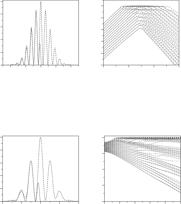
FIGURE 13.9 (a) Probability density at t = 0.3 for the collision of a Gaussian wave packet

with the external potential described by Equation 13.15 (solid line) and another (identical)

Gaussian wave packet under collision-like conditions (dashed line) [44]. To compare, the max-

ima at x ≈−0.32 of both probability densities are normalized to the same height. (b) Bohmian

trajectories illustrating the dynamics associated with the two cases displayed in part (a).

1.0(a) (b)

–5

–10

–15

–20

0.8

0.6

ρ(x,t)

0.4

0.2

0.0

–20 –10 0

x (a.u.)

t (a.u.)

012345

10 20

FIGURE 13.10 (a) Probability density at t = 5 for the collision of a Gaussian wave packet

with the external, time-dependent potential described by Equation 13.24 (solid line) and another

(identical) Gaussian wave packet under diffraction-like conditions (dashed line) [44]. To com-

pare, the maxima at x ≈−5 of both probability densities are normalized to the same height.

(b) Bohmian trajectories illustrating the dynamics associated with the two cases displayed in

part (a).

where x

= x

−v

t (for simplicity, the time-dependent prefactor is neglected, since

it does not play any important role regarding either the probability density or the

quantum trajectories). The probability density associated with Equation 13.16 is

ρ(x, t ) ∼ e

−(x+x

)/2σ

+ e

−(x−x

)/2σ

+ 2e

−(x

)/2σ

cos

[

f (t)x

]

, (13.17)

212 Quantum Trajectories

with

f (t) ≡

t

2mσ



. (13.18)

As can be noticed, Equation 13.17 is maximum when the cosine is +1 (construc-

tive interference) and minimum when it is −1 (destructive interference). The ﬁrst

minimum (with respect to x = 0) is then reached when f (t)x = π, i.e.,

min

(t) =



t

2mσ

πσ

2pσ



t

2mσ

, (13.19)

for which

ρ[x

min

(t)]∼4e

−(x

min

)/2σ

sinh



min

2σ



, (13.20)

which is basically zero if the initial distance between the two wave packets is relatively

large compared with their spreading.

In Figure 13.11a, we can see the function x

min

(t) for different values of the prop-

agation velocity v

. As seen, x

min

(t) decreases with time up to a certain value, and

then increases again, reaching linear asymptotic behavior. From Equation 13.19 we

ﬁnd that the minimum value of x

min

(t) is reached at

min

4mσ







−p +

+ p









. (13.21)

–1

min

(t) (a.u.)

(a.u.)

(a) (b)

t (a.u.)

345

012

t (a.u.)

345

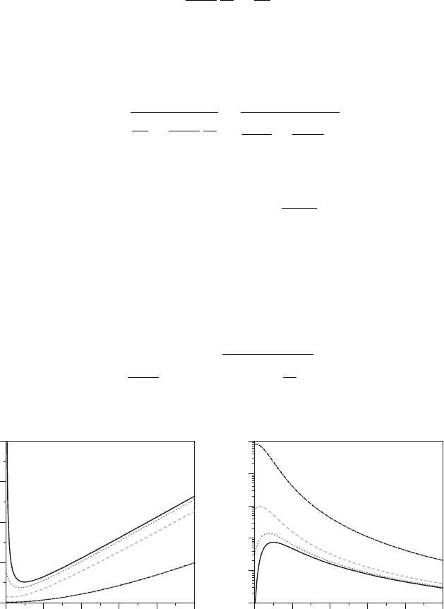
FIGURE 13.11 (a) x

min

as a function of time for different values of the propagation velocity:

= 0.1 (solid line), v

= 2 (dotted line), v

= 10 (dashed line) and v

= 100 (dash-dotted

line). (b) V

as a function of time for the same four values of v

considered in panel (a). In all

cases, v

= 1.

Quantum Interference from a Hydrodynamical Perspective 213

The linear time-dependence at long times is characteristic of the Fraunhofer regime,

where the width of the interference peaks increases linearly with time. On the other

hand, the fact that, at t = 0, x

min

(t) increases as v

decreases (with respect to v

)

could be understood as a “measure” of the coherence between the two wave packets,

i.e., how important the interference among them is when they are far apart (remember

that, despite their initial distance, there is always an oscillating term in between due to

their coherence [42]). In connection with the standard quantum–mechanical argumen-

tation, the diffraction-like features can be associated with the wave nature of particles,

while collision-like ones will be related to their corpuscular nature (they behave more

classical-like). Thus, as the particle becomes more “quantum–mechanical,” the initial

reaching of the “effective” potential well should be larger, whereas, as the particle

behaves in a more classical fashion, this reach should decrease and be only relevant

near the scattering or interaction region, around x = 0. From Equation 13.19, two

limits are thus worth discussing. In the limit p ∼ 0,

min

(t) ≈

πσ

(13.22)

and t

min

≈ τ. In the long-time limit, this expression becomes x

min

(t) ≈ (π/2m)

(t/x

), i.e., x

min

increases linearly with time, as mentioned above. On the other hand,

in the limit of large σ

(or, equivalently, v

 v

min

(t) ≈

π

(13.23)

and t

min

≈ 0. That is, the width of the “effective” potential barrier remains constant

in time, thus justifying our former hypothesis above, in the scattering-like process,

when we considered w ∼ π/2p.

After Equation 13.19, the time-dependent “effective” potential barrier is deﬁned

as Equation 13.15,

V (t ) =







0 x<x

min

(t)

−V

min

(t)] x

min

(t) ≤ x ≤ 0

∞ 0 <x,

(13.24)

with the (time-dependent) well depth being

min

(t)]=

2

min

(t)

. (13.25)

The variation of the well depth with time is plotted in Figure 13.11a for the different

values of v

considered in Figure 13.11b.As seen, the well depth increases with v

(in

the same way that its width, x

min

, decreases with it) and decreases with time. For low

values of v

, there is a maximum, which indicates the formation of the quasi-bound

state that will give rise to the innermost interference peak (with half the width of the

remaining peaks, as shown in Figure 13.10a). Note that, despite the time-dependence

of the well depth, in the limit v

 v

, we recover Equation 13.14.