Chattaraj P.K. (Ed.) Quantum Trajectories

Подождите немного. Документ загружается.

Bipolar Quantum

Trajectory Methods

Bill Poirier

CONTENTS

15.1 Introduction.................................................................................................235

15.2 The Bipolar Decomposition........................................................................238

15.3 Stationary Bound States in 1D....................................................................239

15.4 Stationary Scattering States in 1D ..............................................................242

15.5 Wavepacket Scattering Dynamics in 1D.....................................................243

15.6 Wavepacket Scattering Dynamics in Many Dimensions ............................246

15.7 Numerical Implementations........................................................................246

15.8 Conclusions.................................................................................................248

Bibliography ..........................................................................................................249

15.1 INTRODUCTION

Over the last two decades, classical trajectory simulations (CTS) [1] have emerged

as the method of choice, for computing the dynamics of atomic nuclei in molecular

and condensed matter systems. Such methods are relatively easy to implement, scale

linearly or quadratically in the number of atoms, and can be trivially parallelized

across many cores of a supercomputing cluster or grid. On the other hand, quan-

tum dynamical effects (tunneling, dispersion, interference, zero-point energy, etc.)

are known or suspected to be important for many systems of current interest, and

there is a demand for reliable numerical methods that treat quantum effects well. This

has motivated a host of theoretical and computational improvements, e.g., mixed

quantum-classical methods [2], semiclassical methods [3,4], centroid dynamics [5],

and trajectory surface hopping (TSH) [6,7], all of which are designed, in principle, to

handle large and complex systems of the sort routinely treated using CTS [1]. How-

ever, as these methods all treat quantum effects only approximately, and generally

do not enable systematic convergence to the exact quantum result, it remains a vital

but largely unanswered question to what extent, and for which applications, these

methods actually capture the relevant quantum dynamical effects for the system in

question [8].

The “conventional wisdom” states that more accurate methods, i.e., those that

better represent quantum effects, require substantially greater computational (CPU)

effort. However, this is not necessarily the case. For TSH for instance, one type of

235

236 Quantum Trajectories

quantum effect—i.e., nonadiabatic transitions (essential for processes such as elec-

tron transfer)—is treated almost exactly, for a CPU cost comparable to a CTS [6,7].

This is because TSH employs CTS to propagate a molecular system on a single

potential energy surface (PES) at a time, treating nonadiabatic transitions via random

“hops” from one PES to another. Thus, if other quantum effects are small—e.g., in

the classical limit of large action (mass and/or energy) for which CTS is presumed

valid—then TSH can provide remarkably accurate results, even for pronounced inter-

surface coherences [6,7]. The TSH situation above suggests that highly accurate and

numerically efﬁcient quantum dynamical methods are attainable, perhaps even for

single-PES dynamics. Quantum trajectory methods (QTMs) [9–13]—i.e., CTS-like

simulations involving ensembles of trajectories, based (either “purely” or loosely)

on the de Broglie–Bohm formulation of quantum mechanics [14–18]—are proving

to be one such strategy, having already been applied successfully to model systems

with hundreds of dimensions [12,13] (provided curvilinear coordinates are used, and

interference is ignored). In the pure Bohm QTM formulation, the quantum trajectories

are uniquely determined by the exact quantum wavefunction, ψ(x,t), and (essentially)

vice versa; thus, the method is, in principle, exact. Moreover, the fact that differen-

tial probability [e.g., in one dimension (1D), ρ(x,t) dx, as opposed to the probability

density, ρ(x,t) =|ψ(x,t)|

] is conserved along quantum trajectories implies that these

go to precisely where they are needed most, and is what renders large-dimensional

(large-D) computations feasible. Other properties of pure Bohm quantum trajectories

are discussed elsewhere in this book, and in other sources [12,17].

This chapter is concerned with an alternate to the pure Bohm version of QTM,

called the “bipolar” QTM approach [12,19–32]. The bipolar approach is motivated

by a very simple question: What happens to pure Bohm quantum trajectories in the

classical limit?—i.e., the limit in which the mass, m, or the energy, E, of the problem

becomes large. Intuitively, the expected answer is very clear: in the classical limit,

quantum trajectories should approach corresponding classical trajectories, a speciﬁc

manifestation of the more general “correspondence principle,” often invoked in the

theory of quantum mechanics. Of the various quantum dynamical effects described

in the ﬁrst paragraph above, all but one are effects that disappear smoothly, in the

classical limit. For systems that exhibit only these quantum effects, one ﬁnds that pure

Bohm quantum trajectories do indeed approach classical trajectories in the classical

limit, exactly as desired.The manner in which pure Bohm quantum trajectories deviate

from classical behavior as these quantum effects (tunneling, dispersion, and zero-point

energy) are “turned on” is well-understood, and widely regarded to be an elegant

aspect of the Bohmian approach.

On the other hand, there is one exception to the above correspondence rule, and it

is a very important one: interference. Speciﬁcally, for systems that exhibit substantial

reﬂective interference, such as the 1D barrier scattering system of Figure 15.1, the pure

Bohm quantum trajectories do not approach classical trajectories in the classical limit,

and in fact, tend to deviate increasingly from classical behavior in this limit [12,17].

This is a serious concern for real molecular scattering applications, even in many

dimensions, for which, e.g., Figure 15.1 represents the effective 1D “reaction proﬁle”

for a direct chemical reaction. The interference effect can be described as follows.

Bipolar Quantum Trajectory Methods 237

Eckart potential

V(x) = V

sech

(αx)

Transition state

...

Reactants

A + B–C

Incident

wave

Transmitted

wave

Reflected

wave

Products

A–B + C

Reaction coordinate

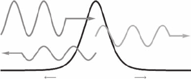
FIGURE 15.1 Schematic indicating a symmetric 1D reactive scattering barrier PES, repre-

senting a reaction proﬁle for a typical direct chemical reaction, A + BC (reactants) → AB + C

(products). The solid black curve indicates the PES, of standard Eckart form [V(x) = V

sech

(αx)]. The upper left sinusoidal curve indicates the left-incident plane wave, ψ

(x), mov-

ing to the right. Quantum mechanically, this is split into a transmitted wave on the far side of the

barrier also moving to the right [also ψ

(x)], and a reﬂected wave, headed to the left [ψ

−

(x),

lower left sinusoidal curve], for energies, E, both above and below the barrier height, V

Classically, E > V

leads to 100% transmission, whereas E < V

leads to 100% reﬂection.

For classical trajectory evolution, there can be only two outcomes: if E is above the

barrier, then all “reactant” trajectories incident on the barrier propagate smoothly to

the far “product” side; if E is below the barrier, then all trajectories are reﬂected by the

barrier, and then head back toward the reactant side. Quantum scattering systems, in

contrast, exhibit partial transmission and reﬂection of the incident wave, both above

and below the barrier. As the incident wave is scattered by the barrier, the reﬂected

portion interferes with the incident wave headed in the opposite direction—leading

to (potentially) strong oscillations in ρ(x,t), which via probability conservation, must

in turn lead to strong, nonclassical oscillations in the quantum trajectories. Moreover,

since the quantum wavelength decreases in the classical limit, the corresponding

oscillations become more pronounced, rather than less, in this limit.

Is it possible, therefore, to deﬁne a new kind of QTM, which has all of the same

advantages as the pure Bohm QTM, yet which also achieves classical correspondence

when there is substantial reﬂection interference? Such a theory would go a very long

way toward justifying the validity of CTS in the classical limit, and perhaps also

generating new and better approximate numerical methods. Such a theory might also

allow exact QTM calculations to be performed in a more classical-like manner, thus

bypassing the infamous “node problem” known to plague pure Bohm QTMs in the

presence of strong interference [12]. Such a theory is the theory of the bipolar QTM.

Interference is an inherently wave-based phenomenon, and therefore cannot be

directly described via a classical trajectory approach—even though it is a quantum

effect that can persist in the classical limit. Nevertheless, the theory of waves, as

applied to both electromagnetism (EM) and quantum scattering, does indeed offer a

238 Quantum Trajectories

classical-like description of interference, through the use of the superposition princi-

ple. Speciﬁcally, interference is regarded as arising from the linear superposition of

two or more wave components, each of which exhibits smooth, interference-free (ide-

ally local plane-wave) behavior. Trajectory descriptions of the resultant components

then exhibit classical-like behavior—e.g., superposed ray optics, in the EM case.

For many quantum reactive scattering applications, such as direct chemical reac-

tions, two components are appropriate: one to represent the forward-reacting wave

(i.e., moving from left to right in Figure 15.1), and the other describing the reverse

(right-to-left) reaction, moving in the opposite direction. A “bipolar” decomposition

of the wavefunction is thus indicated, i.e.,

ψ = ψ

+ ψ

−

, (15.1)

where ψ

describes both the incident and transmitted (product) waves (as these

are both positive-velocity contributions, moving to the right), and ψ

−

describes the

reﬂected (negative-velocity) wave component. The latter comes into being as a result

of incident wave scattering off of the PES barrier; it therefore has vanishing prob-

ability density in the product (right) asymptote. Ideally, the two components, ψ

are themselves interference-free, but otherwise behave as much like a true wavefunc-

tion, ψ, as possible. Separate application of the standard Bohmian prescription to each

of the ψ

would then yield two (sets of) quantum trajectories, each satisfying classical

correspondence automatically. This is the essence of the bipolar QTM approach.

15.2 THE BIPOLAR DECOMPOSITION

The conceptual and potential numerical advantages of the bipolar QTM approach are

clear at the outset. In practice however, there is an immediate difﬁculty to be dealt with:

namely, how does one actually deﬁne the bipolar decomposition of Equation 15.1?The

true wavefunction, ψ itself, is of course presumed to satisfy the Schrödinger equation

(SE), either the time-independent (TISE) or the time-dependent (TDSE) version. The

corresponding pure Bohm quantum trajectory ensemble is then uniquely speciﬁed,

based on the following facts (assuming 1D, for convenience) [12,17]:

1. One quantum trajectory from the ensemble passes through each point in

space, x, at every point in time, t.

2. The velocity of the quantum trajectory passing through the point (x,t) [i.e.,

v(x,t)] is obtained from the phase of ψ(x,t) [i.e., S(x,t)/h], via

mv(x,t) = S



(x,t), (15.2)

where the prime denotes spatial differentiation.

3. The trajectory evolution can also be described via a quantum version of

Newton’s second law, i.e.,

m ¨x = m ˙v =−V



eff

(x, t ) =−[V



(x) + Q



(x, t )] (15.3)

where V (x) is the PES, and Q(x,t) =−(h

/2m)|ψ|



/|ψ|the “quantum poten-

tial” [12,15–17].

Bipolar Quantum Trajectory Methods 239

Thus, the pure Bohm, or “unipolar” equations of motion are known a priori, and QTM

development in this approach is essentially all numerical. In the bipolar approach,

however, before any such numerical progress can be made, one must ﬁrst arrive at

a suitable deﬁnition for the ψ

components. To this end, Equation 15.1 per se is

of little direct help, as it admits an inﬁnite-dimensional range of solutions. Clearly,

additional considerations must be brought into play. In this chapter, we discuss a

particular bipolar strategy based on classical correspondence [19–25], although there

are clearly other, potentially very different approaches that can also be taken, such as

the covering function method of Wyatt and coworkers [26].

For the present, classical correspondence-based bipolar approach, we ﬁnd it con-

venient to start with the simplest case imaginable, i.e., stationary bound state solutions

of the 1D TISE, and then work in stages up to multidimensional TDSE wavepacket

scattering.

15.3 STATIONARY BOUND STATES IN 1D

For stationary bound states in one (Cartesian) dimension, x, the TISE eigenstate solu-

tions, ψ(x), are L

-integrable (

∫

ρ(x)dx = 1), and can be taken to be real-valued

for all x. Together with Equation 15.1, this essentially implies that ψ

(x) must be

complex conjugates of each other. Thus, ρ

(x) = ρ

−

(x), and (from Equation 15.2

above) v

(x) =−v

−

(x) for all x, whereas v(x) = 0 for ψ(x) itself. One can therefore

regard ψ(x) as a “standing wave,” constructed from a linear superposition of two

equal and opposite “travelling waves,” i.e., the two bipolar components, ψ

(x). The

standing wave ψ(x) can be highly oscillatory and nodal, which is certainly the case

for the highly-energetically-excited eigenstates—i.e., in the classical limit of large E.

However, the desired bipolar components, ψ

(x), should be smooth and nonoscilla-

tory across all energies; moreover, the associated bipolar quantum trajectories should

approach the corresponding classical trajectories, in the large-E limit. Finally, the

(x) components should themselves resemble TISE solutions as much as possible,

and in particular, must lead to bipolar densities, ρ

(x), that are also stationary (i.e.,

that exhibit no time dependence, when Equation 15.1 and the TISE are inserted into

the TDSE).

In attempting to achieve all of the above requirements, a natural ansatz is to presume

(x) components that are themselves mathematical TISE solutions, for the same E

as ψ(x) itself. Of course, these ψ

(x) cannot be physical TISE solutions, as they are

non-L

-integrable, and exhibit ρ

(x) densities that diverge in both left- and right-

asymptotic limits. However, this choice is certainly stationary and node-free, and

TISE-solution-like. Moreover, the set of all possible bipolar decompositions has now

been reduced from an inﬁnite-parameter space to a two-parameter space, since the

TISE admits two linearly-independent solutions. The two parameters are complex-

valued; however, one of these is associated with the overall scaling and phase of

ψ(x) itself, which as discussed above, is already predetermined. This leaves one

complex-valued parameter, or alternatively, two real-valued parameters, that must

still be determined.

240 Quantum Trajectories

The remaining two real-valued parameters will be chosen such that the resultant

bipolar quantum trajectory ensembles, i.e., the velocity ﬁelds, v

(x), resemble the

corresponding classical trajectory ensembles as closely as possible [19]. To this end,

it is encouraging to note that the classical trajectory ensembles for bound 1D systems

are indeed also bipolar (i.e., are characterized by double-valued velocity ﬁelds for

classically allowed x values), with equal and opposite velocities given by

=±



2[E − V (x)]/m. (15.4)

One therefore expects v

(x) to be chosen, such that |v

(x)-v

(x)| or |Q

(x)| is mini-

mized over the classically allowed region, V(x) < E, and also, such that these quan-

tities vanish in the classical limit of large E. Such a choice is possible, as discussed

below. In contrast, the unipolar, pure Bohm QTM approach, always gets the physics

wrong, because it is incapable of predicting both a positive- and negative-velocity

value at a given point x—instead predicting their average value, v(x) = 0, which is

increasingly inaccurate in the large E limit. This situation is very reminiscent of the

well-known failure of Ehrenfest dynamics when applied to multisurface systems, for

which a single, averaged dynamical propagation across all PESs is predicted, rather

than separate propagations on each individual PES. Indeed, the latter consideration

has led to the development of the much-superior, TSH approach for nonadiabatic

dynamics [6,7]; a similar TSH scheme for bipolar propagation on a single-PES will

be discussed later in this chapter (Section 15.7).

To characterize the family of available TISE solutions, the two real parameters are

taken to be [19]:

1. The absolute value of the bipolar ﬂux, F =|ρ

(x)v

(x)|,anx-independent

constant.

2. The median of the enclosed action, x

deﬁned such that

∫

(x)dx =

∫

(x)dx =±(πh/2)(n +1),

where n denotes the excitation number of the particular energy eigenstate, starting

with n = 0 as the ground state. It is helpful to consider the phase space portraits of the

relevant trajectory orbits, as is done in Figure 15.2 for the simple harmonic oscillator

example, V(x) = (k/2)x

, with k = m = 1. Classically, the v

and v

−

orbits for a given

n form a closed loop, encircling a half-integer-quantized phase space volume (action)

equal to 2πh(n + 1/2) (the circular curves in Figure 15.2). The associated quantum

trajectories extend across all x, but always enclose a ﬁnite, and integer-quantized

phase space volume of 2πh(n + 1), regardless of the particular choice of F and

parameters. Moreover, by choosing F and x

to equal the corresponding classical

values, one obtains bipolar quantum trajectories (the eye-shaped curves in Figure 15.2)

that are nearly indistinguishable from their classical counterparts in the classically

allowed region of space, and in the classical limit.As indicated in Figure 15.3, it is also

true that Q

(x) → 0 in this region; however, in order to avoid turning points, Q

(x)

becomes large and negative in the classically forbidden asymptotes, thus ensuring

that V

eff

(x) < E and v

(x) > 0 for all x, where

=±



2[E − V

eff

(x)]/m. (15.5)

Bipolar Quantum Trajectory Methods 241

–6.0

5.0

3.0

1.0

–1.0

–3.0

–5.0

–4.0 –2.0 0.0

Position x

Momentum p(x)

2.0 4.0 6.0

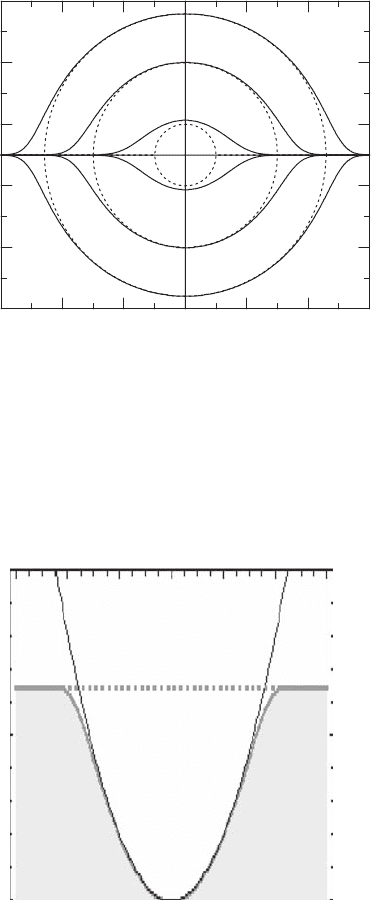
FIGURE 15.2 Phase space orbits for bipolar quantum trajectories for three different harmonic

oscillator eigenstates; moving concentrically outward from the origin, these are n = 0, n = 4,

and n = 10, respectively. Solid curves indicate bipolar quantum trajectories; dotted curves

indicate corresponding classical trajectories. The correspondence principle is clearly satisﬁed

with increasing n. (Reprinted with permission from Poirier, B., Journal of Chemical Physics,

121, 4501–4515, 2004.)

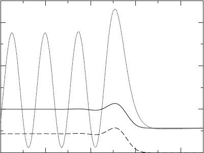
FIGURE 15.3 Bipolar effective potential, V

eff

(x) (thick solid curve), and true potential,

V(x) (thin solid curve), for the sixth excited harmonic oscillator eigenstate, n = 6. Note that

eff

(x) < E everywhere, where the eigenenergy, E, is indicated by the thick dashed horizontal

line. In the classically allowed region, V

eff

(x) ≈ V(x), but V

eff

(x) ≈ E in the classically forbid-

den region. (Modiﬁed from Poirier, B., Journal of Chemical Physics, 121, 4501–4515, 2004.

With permission.)

242 Quantum Trajectories

15.4 STATIONARY SCATTERING STATES IN 1D

For stationary scattering states in 1D, i.e., the continuum TISE eigenstate solu-

tions, the situation is substantially more complicated. First, there are no L

-integrable

solutions, and so for any given E, the two linearly-independent mathematical solutions

(and arbitrary superpositions) are both physically allowed. Without loss of general-

ity, we restrict consideration to the left-incident solution ψ(x), only. Assuming for

simplicity that V(x) → 0 in both asymptotes, then in order to avoid interference and

match classical behavior asymptotically, clearly ψ

(x) ∝ exp[ikx] in both asymp-

totes, and ψ

−

(x) ∝ exp[−ikx] in the left asymptote, where (h

/2m) = E. However,

it can be shown that there are no TISE solutions ψ

(x) that satisfy these asymptotic

conditions, which is the primary difﬁculty for the stationary scattering generalization

of the bipolar theory. In order to achieve classical correspondence, therefore, we must

consider non-TISE ψ

(x)’s.

It is a well-known fact of scattering theory that for a given TISE solution, the

ﬂux of the incident stream is equal to the sum of the reﬂected and transmitted stream

ﬂux absolute values. Thus, the ﬂux, F

, associated with say, ψ

(x), far from being

an x-independent constant, must decrease from the left asymptote [where ψ

(x) rep-

resents the incident wave] to the right [where it represents the transmitted wave]. The

decrease in F

is matched by an increase in F

−

for the reﬂected wave, ψ

−

(x), and is

associated with dynamical coupling between the two components—a manifestation

of scattering induced by the PES barrier. This dynamical coupling occurs only in

the PES barrier region of x, i.e., where V(x) is nonzero, and serves to induce tran-

sitions (or probability ﬂow) between the two bipolar components. Borrowing from

semiclassical theory [3], this leads to a unique Equation 15.1 decomposition for a

given effective potential, V

eff

(x), where the resultant ψ

(x) are guaranteed to exhibit

the correct asymptotic behavior [20–22]. However, the determination of V

eff

(x)in

this formalism is unspeciﬁed, unlike in Section 15.3. The simplest possible choice is

eff

(x) = 0, leading to the following dynamical equations [20–22]:

dψ







(E − V )ψ

−







V ψ

∓

(15.6a)

∂ρ

∂t

=−F





Im[ψ

∗

−

] (15.6b)

with (d/dt) denoting total time derivative. These equations are time-dependent, but

guaranteed to converge to the correct TISE stationary solution in the large-time limit.

Equation 15.6b implies the important, nontrivial property that total probability for

both components is conserved (related to the stream ﬂux property described above),

which is also true for other choices of V

eff

(x).

Figure 15.4 indicates the bipolar and unipolar solution densities, for a standard

symmetric 1D benchmark PES (the Eckart barrier of Figure 15.1), for the choice

eff

(x) = 0. Unlike ρ(x), which necessarily exhibits reﬂective interference in the

left asymptote, both of the bipolar densities, ρ

(x), are constant in both asymptotes,

as expected. For this particular system, ρ

(x) are also smooth and nonoscillatory in

Bipolar Quantum Trajectory Methods 243

−3 −2 −1 0 1

Position, x

0.0

1.0

2.0

3.0

Density, ρ(x)

−

FIGURE 15.4 Computed unipolar and bipolar probability densities, for TISE energy eigen-

state of the Eckart barrier system of Figure 15.1, with E = V

. Solid curve: bipolar ρ

(x);

dashed curve: bipolar ρ

−

(x); dotted curve: unipolar ρ(x). The latter exhibits pronounced reﬂec-

tion interference in the left asymptote, but the bipolar curves are ﬂat in both asymptotes.

The transmission and reﬂection probabilities, i.e., right and left asymptotic values of ρ

(x)

and ρ

−

(x), respectively, are roughly equal. (Modiﬁed from Poirier, B., Journal of Chemical

Physics, 124, 034116, 2006. With permission.)

the barrier region, as desired. However, it can be shown that in the classical limit as

m →∞, and/or E (and V

, the barrier height) →∞, then the choice V

eff

(x) = 0 leads

to barrier region oscillations in ρ

(x), particularly when the reaction proﬁle has a PES

well (reaction intermediate, i.e., nondirect reaction). Intuitively, the reason for this

undesirable behavior is clear: based on the discussion in Section 15.3, the appropriate

effective potential should have V

eff

(x) ≈ V(x) in the classically allowed region, and—

for below barrier energies—V

eff

(x) ≈ E in the barrier tunneling region. Indeed, ad

hoc construction of such V

eff

(x) effective potentials always leads to improved (i.e.,

nonoscillatory) ρ

(x) behavior, which is very useful for practical applications. At the

present stage of development, however, there does not exist a means to single out

a unique V

eff

(x) a priori, as is the case for the stationary bound states, though this

is an active area of ongoing investigation. This issue will resurface again in various

contexts.

15.5 WAVEPACKET SCATTERING DYNAMICS IN 1D

The next generalization of the bipolar decomposition to be derived is for 1D TDSE

wavepacket scattering dynamics. This is an essential prerequisite for generalization to

large-D QTM calculations, for which the favorable numerical scaling requires wave-

functions that are well-localized in space, for all relevant times. The TISE scattering