Engelbrecht Andries P. Computational Intelligence: An Introduction

Подождите немного. Документ загружается.

558 A. Optimization Theory

Algorithm A.2 summarizes the SA algorithm. The algorithm requires speciﬁcation of

the following components:

• A representation of possible solutions, which is usually a vector of ﬂoating-

point values.

• A mechanism to generate new solutions by adding small random changes

to current solutions. For example, for continuous-valued vectors,

x(t +1)=x(t)+D(t)r(t)(A.6)

where r(t) ∼ U (−1, 1)

,andD is a diagonal matrix that deﬁnes the maximum

change allowed in each variable. When an improved solution is found,

D(t +1)=(1− α)D(t)+αωR(t)(A.7)

where R(t) is a diagonal matrix whose elements are the magnitudes of the suc-

cessful changes made to each variable, and α and ω are constants.

For integer problems,

x(t +1)=x(t)+r(t)(A.8)

where each element of r(t) is randomly selected from the set {−1, 0, 1}.

• A method to evaluate solutions, which is usually just the objective function

in the case of unconstrained problems.

• An annealing schedule, which consists of an initial temperature and rules for

lowering the temperature with increase in number of iterations. The annealing

schedule determines the degree of uphill movement (objective function increase)

allowed during the search. An initial high temperature is selected, which is then

incrementally reduced using, for example,

– Exponential cooling: T (t +1)=αT (t), where α ∈ (0, 1).

– Linear cooling: T (t+1) = T (t)−∆T ,where,e.g. ∆T =(T (0)−T (n

))/n

;

T (0) is the initial large temperature, and T (n

) is the ﬁnal temperature at

the last iteration, n

Algorithm A.2 Simulated Annealing Algorithm

Create initial solution, x(0);

Set initial temperature, T (0);

t =0;

repeat

Generate new solution, x;

Determine quality, f(x);

Calculate acceptance probability using equation (A.5);

if U(0, 1) ≤ acceptance probability then

x(t)=x;

end

until stopping condition is true;

Return x(t) as the solution;

A.5 Unconstrained Optimization 559

LeapFrog Algorithm

LeapFrog is an optimization approach based on the physical problem of the motion

of a particle of unit mass in an n

-dimensional conservative force ﬁeld [799, 800]. For

more detail refer to Section 3.2.4.

A.5.3 Example Benchmark Problems

This section lists a number of the classical benchmark functions used to evaluate the

performance of optimization algorithms for unconstrained optimization. The purpose

of the section is not to provide an extensive list of example problems, but to provide

a list that can be used as a good starting point when analyzing the performance of

optimization methods.

Spherical:

f(x)=



j=1

(A.9)

with x

∈ [−100, 100] and f

∗

(x)=0.0.

Quadric:

f(x)=



j=1





k=1



(A.10)

with x

∈ [−100, 100] and f

∗

(x)=0.0.

Ackley:

f(x)=−20e

−0.2





j=1

−e



j=1

cos(2πx

)

+20+e (A.11)

with x

∈ [−30, 30] and f

∗

(x)=0.0.

Bohachevsky 1:

f(x

)=x

+2x

− 0.3cos(3πx

) − 0.4cos(4πx

)+0.7 (A.12)

with x

∈ [−50, 50] and f

∗

)=0.0.

Colville:

f(x

) = 100(x

− x

)

+(1− x

)

+ 90(x

− x

)

+(1 − x

)

+10.1((x

− 1)

+(x

− 1)

)

+19.8(x

− 1)(x

− 1) (A.13)

with x

∈ [−10, 10] and f

∗

)=0.0.

Easom:

f(x

)=−cos(x

) cos(x

−(x

−π)

−(x

−π)

(A.14)

with x

∈ [−100, 100] and f

∗

)=−1.0.

560 A. Optimization Theory

Griewank:

f(x)=1+

4000



j=1

−



j=1

cos



√



(A.15)

with x

∈ [−600, 600] and f

∗

(x)=0.0.

Hyperellipsoid:

f(x)=



j=1

(A.16)

with x

∈ [−1, 1] and f

∗

(x)=0.0.

Rastrigin:

f(x)=



j=1

− 10 cos(2πx

) + 10) (A.17)

with x

∈ [−5.12, 5.12] and f

∗

(x)=0.0.

Rosenbrock:

f(x)=



j=1

[100(x

− x

2j−1

)

+(1− x

2j−1

)

] (A.18)

with x

∈ [−2.048, 2.048] and f

∗

(x)=0.0.

Schwefel:

f(x)=



j=1

sin







+ 418.9829n

(A.19)

with x

∈ [−500, 500] and f

∗

(x)=0.0.

A.6 Constrained Optimization

Many real-world optimization problems are solved subject to sets of constraints. Con-

straints place restrictions on the search space, specifying regions of the space that are

infeasible. Optimization algorithms have to ﬁnd solutions that do not lie in infeasi-

ble regions. That is, solutions have to satisfy all speciﬁed constraints. This chapter

provides a mathematical deﬁnition of the constrained optimization problem in Sec-

tion A.6.1. An overview of constraint handling methods is given in Section A.6.2.

Section A.6.3 provides a list of benchmark functions.

A.6.1 Problem Deﬁnition

Assuming a minimization problem, the general constrained problem is deﬁned as:

A.6 Constrained Optimization 561

Definition A.5 Constrained optimization problem:

minimize f(x), x =(x

,...,x

)

subject to g

(x) ≤ 0,m=1,...,n

(x)=0,m= n

+1,...,n

+ n

∈ dom(x

) (A.20)

where n

and n

are the number of inequality and equality constraints respectively,

and dom(x

) is as defined in Section A.5.1.

A special instance of the constrained optimization problem is deﬁned below, where

only linear equality constraints of the form Ax = b are deﬁned:

Definition A.6 Constrained optimization with linear equality constraints:

minimize f(x), x =(x

,...,x

)

subject to Ax = b (A.21)

where A ∈ R

×n

and b ∈ R

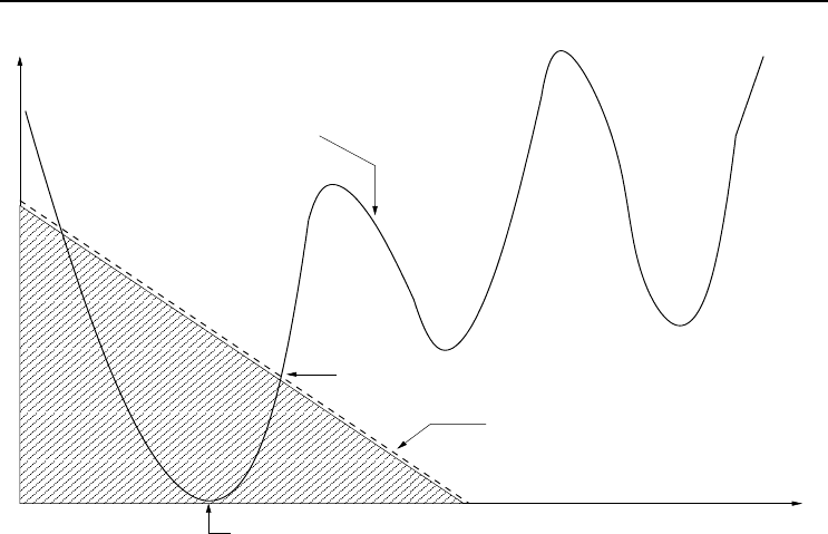
Figure A.3 illustrates the eﬀect of constraints. The shaded area indicates the infea-

sible region of the search space. Note how the global optimum for the unconstrained

function is no longer the global optimum for the constrained problem. Instead, the

best solution is an extremum (not called an optimum, since the derivative of the best

solution is not zero).

A.6.2 Constraint Handling Methods

The following types of constraints can be found:

• Boundary constraints, which basically deﬁne the borders of the search space.

Upper and lower bounds on each dimension of the search space deﬁne the hy-

percube in which solutions must be found. While boundaries are usually deﬁned

by specifying upper and lower bounds on variables, such box constraints are not

the only way in which boundaries are speciﬁed. The boundary of a search space

can, for example, be on the circumference of a hypersphere. It is also the case

that a problem can be unbounded.

• Equality constraints specify that a function of the variables of the problem

must be equal to a constant.

• Inequality constraints specify that a function of the variables must be less

than or equal to (or, greater than or equal to) a constant.

Constraints can be linear or nonlinear.

Constraint handling methods have to consider a number of important questions, which

relate mainly to the trade-oﬀ between feasible and infeasible solutions:

562 A. Optimization Theory

Infeasible space

Feasible space

ed G

oba

l Minim

Objective function

Extremum

Inequality constraint

f(x)

Figure A.3 Constrained Problem Illustration

• How should two feasible solutions be compared? The answer to this question is

somewhat obvious: the solution with the better objective function value should

be preferred.

• How should two infeasible solutions be compared? In this case the answer is not

at all obvious, and is usually problem-dependent. The issues to consider are:

– should the infeasible solution with the best objective function value be

preferred?

– should the solution with the least number of constraint violations or lowest

degree of violation be preferred?

– should a balance be found between best objective function value and degree

of violation?

• Should it be assumed that any feasible solution is better than any unfeasible

solution? Alternatively, can objective function value and degree of violation

be optimally balanced? Again, the answer to this problem may be problem-

dependent. In ﬁnancial-critical, or life-critical problems, the ﬁrst strategy should

be preferred to ensure no ﬁnancial loss, or loss of life. Less critical problems,

such as time-tabling, may consider solutions where less severe constraints are

violated.

Research in constraint handling methods are numerous in the evolutionary computa-

tion (EC) and swarm intelligence (SI) paradigms. Based on these research eﬀorts, con-

straint handling methods have been categorized in a number of classes [140, 487, 584]:

A.6 Constrained Optimization 563

• Reject infeasible solutions, where solutions are not constrained to the feasible

space. Solutions that ﬁnd themselves in infeasible space are simply rejected or

ignored.

• Penalty function methods, which add a penalty to the objective function to

discourage search in infeasible areas of the search space.

• Convert the constrained problem to an unconstrained problem,then

solve the unconstrained problem.

• Preserving feasibility methods, which assumes that solutions are initialized

in feasible space, and applies specialized operators to transform feasible solutions

to new, feasible solutions. These methods constrict solutions to move only in

feasible space, where all constraints are satisﬁed at all times.

• Pareto ranking methods, which use concepts from multi-objective optimiza-

tion, such as non-dominance (refer to Section A.8), to rank solutions based on

degree of violation.

• Repair methods, which apply special operators or actions to infeasible solu-

tions to facilitate changing infeasible solutions to feasible solutions.

The rest of this section provides a short deﬁnition and discussion of two of these

approaches.

Penalty Methods

Penalty methods add a function to the objective function to penalize vectors that rep-

resent infeasible solutions. Assuming a constrained minimization problem as deﬁned

in Deﬁnition A.5,

Definition A.7 Penalty method:

minimize F (x,t)=f(x,t)+λp(x,t) (A.22)

where λ is the penalty coefficient and p(x,t) is the (possibly) time-dependent penalty

function.

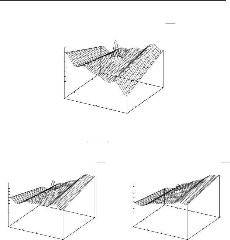
A major problem of penalty-based methods is due to the added penalty function, which

changes the shape of the objective function. While the change in objective function is

necessary to increase the slope of the function in the infeasible areas (assuming min-

imization), the penalty function may introduce false minima into the original search

space as deﬁned by the unpenalized function. These false minima may trap search

algorithms. Figure A.4 illustrates the eﬀect of penalty functions. Figure A.4(a) illus-

trates the function

f(x

cos(x

)

+2e

−x

−(x

−1)

+0.01x

(A.23)

with one clear maximum at x

∗

=(0.0, 0.0). Figure A.4(b) illustrates the penalized

objective,

F (x

)=f(x

)+λp(x

) (A.24)

564 A. Optimization Theory

f(x1,x2)

-10

-5

-10

-5

-1.5

-1

-0.5

0.5

1.5

f(x1,x2)

(a) f(x

cos(x

)

+2e

−x

−(x

−1)

+0.01x

-10

-5

-10

-5

-2.5

-2

-1.5

-1

-0.5

0.5

1.5

2.5

f(x1,x2)

F(x1,x2)

f(x1,x2)

(b) With penalty p(x

)=3x

and λ =0.05

-10

-5

-10

-5

-4

-3

-2

-1

f(x1,x2)

F(x1,x2)

f(x1,x2)

)=3x

and λ =0.1

Figure A.4 Illustration of the Eﬀect of Penalty Functions

where λ =0.05 and p(x

)=3x

. Notice how the penalty causes the slope of the

function to increase for large x

and x

values, with function values exceeding that

of the maximum of the original function f(x

). This eﬀect is for a low penalty

coeﬃcient of λ =0.05. For larger values, the slope increases even more as illustrated

in Figure A.4(c) for λ =0.1.

The penalty function is usually constructed from a set of functions, one for each of the

constraints, quantifying the degree to which a solution violates the constraint. That

A.6 Constrained Optimization 565

is,

p(x

,t)=



m=1

(t)p

) (A.25)

where



max{0,g

)

} if m ∈ [1,...,n

] (inequality)

if m ∈ [n

+1,...,n

+ n

] (equality)

(A.26)

with α a positive constant, representing the power of the penalty. In equation (A.25),

(t) represents a time-varying degree to which violation of the m-th constraint con-

tributes to the overall penalty. More emphasis can therefore be given to crucial con-

straints. The constraint penalty coeﬃcient can of course be static, i.e. λ

(t)=λ

Convert Constrained to Unconstrained Problem

A constrained problem can be converted to an unconstrained problem by deﬁning

the Lagrangian for the constrained problem, and then by maximizing the Lagrangian.

Consider the standard constrained optimization problem as deﬁned in Deﬁnition A.5,

referred to as the primal problem. The constraints in equation (A.20) can be introduced

into the objective function, f , by augmenting it with a weighted sum of the constraint

functions. Let λ

∈ R

be the weights associated with the n

inequality constraints,

and λ

∈ R

be the weights associated with the n

equality constraints.

These vectors, referred to as the Lagrange multiplier vectors, deﬁne the Lagrangian,

L : R

× R

L(x,λ

,λ

)=f(x)+



m=1

(x)+



m=n

(x) (A.27)

The dual problem associated with the primal problem in equation (A.20) is then

deﬁned as

Definition A.8 Dual problem:

maximize

,λ

L(x,λ

,λ

)

subject to λ

≥ 0,m=1,...,n

+ n

(A.28)

If the primal problem is convex over the search space S, then the solution to the

primal problem is the vector x

∗

of the saddle point, (x

∗

,λ

∗

,λ

∗

), of the Lagrangian in

equation (A.27), such that

L(x

∗

,λ

) ≤ L(x

∗

,λ

∗

,λ

∗

) ≤ L(x,λ

∗

,λ

∗

) (A.29)

The vector x

∗

that solves the primal problem, as well as the Lagrange multiplier

vectors, λ

∗

and λ

∗

, can be found by solving the min-max problem,

min

max

,λ

L(x,λ

,λ

) (A.30)

566 A. Optimization Theory

For non-convex problems, the solution of the dual problem does not coincide with the

solution of the primal problem. For non-convex problems, the Lagrangian is augmented

by adding a penalty term, i.e.



(x,λ

,λ

)=L(x,λ

,λ

)+λp(x,t) (A.31)

where λ>0, L(x,λ

,λ

) is as deﬁned in equation (A.27), and the penalty p(x,t)is

as deﬁned in equations (A.25) and (A.26) with λ

(t)=1andα =2.

A.6.3 Example Benchmark Problems

A number of benchmark functions for constrained optimization are listed in this sec-

tion. Again, the list is not intended to be complete. The objective is to provide a list

of constrained problems as a starting point in evaluating algorithms for constrained

optimization.

Constrained problem 1: Minimize the function

f(x) = 100(x

− x

)

+(1− x

)

(A.32)

subject to the nonlinear constraints,

+ x

≥ 0

+ x

≥ 0

with x

∈ [−0.5, 0.5] and x

≤ 1.0. The global optimum is x

∗

=(0.5, 0.25), with

f(x

∗

)=0.25.

Constrained problem 2: Minimize the function

f(x)=(x

− 2)

− (x

− 1)

(A.33)

subject to the nonlinear constraint

−x

+ x

≥ 0

and the linear constraint

+ x

≤ 2

with x

∗

=(1, 1) and f(x

∗

)=1.

Constrained problem 3: Minimize the function

f(x)=5x

+5x

− 5



j=1

−



j=5

(A.34)

subject to the constraints

+2x

+ x

≤ 10 2x

+2x

+ x

≤ 10

+2x

+ x

≤ 10 −8x1+x

≤ 0

−8x

+ x

≤ 0 −8x

+ x

≤ 0

−2x

− x

+ x

0 ≤ 0 −2x

− x

+ x

≤ 0

−2x

− x

+ x

≤ 0

A.7 Multi-Solution Problems 567

with x

∈ [0, 1] for j =1,...,9, x

∈ [0, 100] for j =10, 11, 12, and x

∈ [0, 1].

The solution is x

∗

=(1, 1, 1, 1, 1, 1, 1, 1, 1, 3, 3, 3, 1), with f(x

∗

)=−15.

Constrained problem 4: Maximize the function

f(x)=(

√

)



j=1

(A.35)

subject to the equality constraint,



j=1

with x

∈ [0, 1]. The solution is x

∗

√

,...,

√

), with f(x

∗

)=1.

Constrained problem 5: Minimize the function

−10.5x

− 7.5x

− 3.5x

− 2.5x

− 1.5x

− 10x

− 0.5



j=1

(A.36)

subject to the constraints

+3x

+2x

+ x

− 6.5 ≤ 0

10x

+10x

+ x

≤ 20

with x

∈ [0, 1] for j =1,...,5, and x

≥ 0. The best known solution is

f(x)=−213.0.

A.7 Multi-Solution Problems

Multi-solution problems are multi-modal, containing many optima. These optima

may include more than one global optimum and a number of local minima, or just

one global optimum together with more than one local optimum. The objective of

multi-solution optimization methods is to locate as many as possible of these optima.

A formal deﬁnition is given in Section A.7.1, with diﬀerent algorithm categories listed

in Section A.7.2. Example benchmark problems are given in Section A.7.3.

A.7.1 Problem Deﬁnition

A multi-solution problem is formally deﬁned as follows (assuming minimization):

Definition A.9 Multi-solution problem: Find a set of solutions, X =

∗

, x

∗

,...,x

∗

}, such that each x

∗

∈Xis a minimum of the general optimization

problem as defined in Definition A.5. That is, for each x

∗

∈X,

||f



∗

)|| ≤ (1 + |f (x

∗

)|) (A.37)

where  is, for example, the square root of machine precision.