Farin G. Curves and Surfaces for CAGD. A Practical Guide
Подождите немного. Документ загружается.

142 Chapter 8 B-Spline Curves
B-spline curves are simply the parametric equivalent of (8.15):
L
x(u) =
J2djNf{u),
;=0
Just as the de Casteljau algorithm for Bezier curves is related to the recursion
of Bernstein polynomials, the de Boor algorithm yields a recursion for B-splines.
It is given by
Nf(u) = ^"^^-^ N^Hu) + ^l^±^ZiiN-i(^), (8.16)
w^ith the "anchor" for the recursion being given by
"?<«' iO else
1 if Ui_i <u <Uj
(8.17)
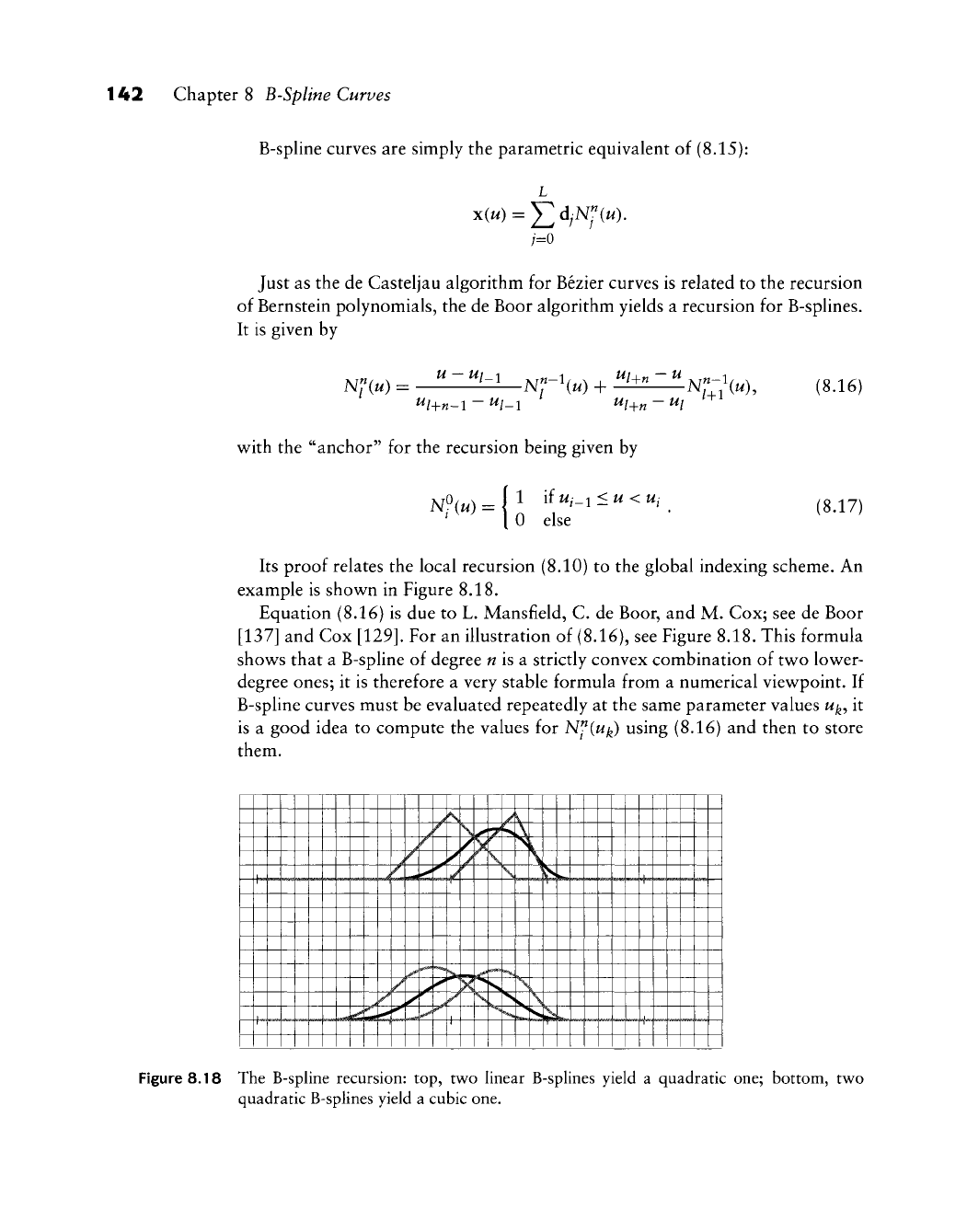
Its proof relates the local recursion (8.10) to the global indexing scheme. An
example is shov^^n in Figure 8.18.
Equation (8.16) is due to L. Mansfield, C. de Boor, and M. Cox; see de Boor
[137] and Cox
[129].
For an illustration of (8.16), see Figure 8.18. This formula
shows that a B-spline of degree
w
is a strictly convex combination of tw^o lower-
degree ones; it is therefore a very stable formula from a numerical viewpoint. If
B-spline curves must be evaluated repeatedly at the same parameter values w^, it
is a good idea to compute the values for N^{uf^) using (8.16) and then to store
them.
T"
-
... ...
«...
A
/_
/
A
V
J\
..„
4
f
ri
««»''<
V
'"
k
>^
+-
\
X
V
*•,
y^.^
\
("•^
k
-
• .
ffM
-
-
-
^.
-'
4.
4-
-
-
...
Figure 8.18 The B-spline recursion: top, two linear B-splines yield a quadratic one; bottom, two
quadratic B-splines yield a cubic one.
8.9 B-Spline Basics 143
A comment on end knot multiplicities: the widespread data format IGES uses
two additional knots at the ends of the knot sequence; in our terms, it adds knots
u_i and ^L+2n-l- The reason is that formulas like (8.16) seemingly require the
presence of these knots. Since they are multiplied only by zero factors, their values
have no influence on any computation. There is no reason to store completely
inconsequential data, and hence the "leaner" notation of this chapter.
8.9 B-Spline Basics
Here, we present a collection of the most important formulas and definitions of
this chapter. As before, n is the (maximal) degree of each polynomial segment,
L + 1 is the number of control points, and K is the number of intervals.
Knot sequence:
{WQ,
...,
Uf^},
Control points: do,..., d^, with L = K -n + 1.
Domain: Curve is only defined over [u^-\^..., u^],
Greville abscissae:
^i
=
^(Uj-\
h
^/-f^-i).
Support: N^ is nonnegative over [w/_i,
^/+„].
Knot insertion: To insert uj <u < w/+i, first find new Greville abscissae |/, then
set new dj = P(|/).
de Boor algorithm: Given uj <u < uj^i^ renumber the relevant control points
d/_^^i,..., Aj^i as do,..., d„ and then set
df
(M)
- (1 - af )df-l(«) + «f df^i^M)
with
for ^ = r + 1,...,
w,
and i = 0,... ,n
—
k. Here, r denotes the multiplicity of
u, (Normally, u is not already in the knot sequence; then, r = 0.)
Mansfield, de Boor, Cox recursion:
Ul+„-l~Ui_^ Ui+„-Ul
144 Chapter 8 B-Spline Curves
Derivative:
-^Nfiu) = N^-\u)
N^-\u),
Derivative of B-spline curve
_d_
Degree elevation:
^»
=
;;^E^rV;^;),
where Nf'^ (u;
Uj)
is defined over the original knot sequence except that the
knot
Uj
has its muhiphcity increased by one. This identity was discovered by
H. Prautzsch in 1984
[493].
Another reference is Barry and Goldman [39].
8.10 Implementation
Here is the header for the de Boor algorithm code:
float deboor(degree,coeff,knot,u,i)
/*
uses
de
Boor algorithm
to
compute
one
coordinate
on
B-spline curve
for
param. value
u in
interval
i.
Input: degree: polynomial degree
of
each piece
of
curve
coeff: B-spline control points
knot: knot sequence
u: evaluation abscissa
i:
u's
interval: u[i]<=
u <
u[i+l]
Output: coordinate value.
V
This program does not need to know about L. The next program generates a
set of points on a whole B-spline curve—for one coordinate, to be honest—so it
has to be called twice for a 2D curve and three times for a 3D curve.
bspl_to_points(degree,1,coeff,knot,dense,points,point_num)
/* generates points on B-spline curve, (one coordinate)
Input: degree: polynomial degree of each piece of curve
1:
number of active intervals
8.10 Implementation 145
coeff:
B-spline control points
knot: knot sequence: knot[0].. .knot[l+2*clegree-2]
dense:
how
many points
per
segment
Output:points: output array with function values.
point_num:
how
many points
are
generated. That number
is
easier computed here than
in the
calling program:
no points
are
generated between multiple knots.
V
The main program deboormai
n. c
generates a postscript plot of a B-spline curve.
A sample input file is in bspl .dat; it creates the outline of the letter r from Figure
5.11.
As a second example, the input data for the y-values of the curve in Figure
8.10 are
degree = 3; 1 = 3; coeff = 1,4,4,0,0,1;
knot = 0,0,0,3,9,12,12,12; dense = 10.
Next, w^e include a B-spline blossom routine:
deboor_blossom(control,degree,deboor,deboor_wts,
knot,uvec,i nterval,poi nt,poi nt_wt)
/*
FUNCTION: deBoor algorithm
to
evaluate
a
B-spline curve blossom.
For polynomial
or
rational curves.
INPUT: control[] [0]: indicates type
of
input curve
0
=
polynomial
1
=
rational
[1]:
indicates
if
input/output
is
in
R3 or
R4;
3
= R3
4
= R4
degree polynomial degree
of
each piece
of
the
input curve, must
be
<=20
deboor[][3] deboor control points
deboor_wts[] rational weights associated with
the control points
if
control[0]=1;
otherwise weights
not
used
146 Chapter 8 B-Spline Curves
knot[] knot sequence with multiplicities
entered explicitly
uvec[] blossom (parameter) values
to evaluate
i
nterval
i
nterval
wi thi n
knot sequence
with which
to
evaluate wrt
u
(typically: i=interval then
knot[i]<=
u <
knot[i+l])
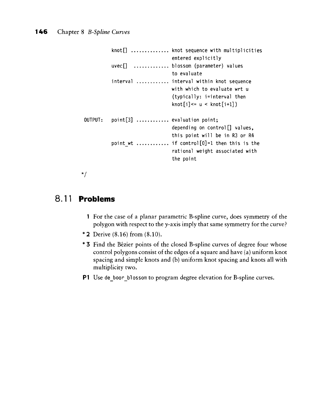
OUTPUT: point [3]
point_wt
evaluation point;
depending on control[] values,
this point will be in R3 or R4
if control[0]=1 then this is the
rational weight associated with
the point
8.11 Problems
1 For the case of a planar parametric B-spHne curve, does symmetry of the
polygon with respect to the y-axis imply that same symmetry for the curve?
Derive (8.16) from (8.10).
Find the Bezier points of the closed B-spline curves of degree four whose
control polygons consist of the edges of a square and have (a) uniform knot
spacing and simple knots and (b) uniform knot spacing and knots all with
multiplicity two.
PI Use de_boor_blossom to program degree elevation for B-spline curves.
*2
*3
Constructing Spline
Curves
/V spline is a flexible rod of wood or plastic. It has its origins in shipbuilding,
where splines were used to draft the curves (ribs) that define a ship body. Early
uses go back to the 1600s, and are documented in
[450].
Although mechanical
splines are used less frequently now, the underlying principle still gives rise to
new algorithms.
9.1 Greville Interpolation
In Chapter 7, we saw how to pass a polynomial curve of degree n through
n
-\-
1 data points Po?
• • • ? Pw
with parameter values
^Q?
• • • ?
^w The key to the
solvability of the problem was simple: the number of knowns (the data points
with parameter values) had to equal the number of unknowns (the polynomial
coefficients).
Something quite analogous happens in a spline context. A spline curve of
degree n is defined over a knot sequence
UQ,
.. .
^
u^^.
Such a knot sequence has
K
—
n-\-2 Greville abscissae ^/ and hence the spline curve has L-^1 = K
—
n-\-2
B-spline control points do,..., d^^.
In view of these numbers, the following is a meaningful interpolation problem:
Given: A knot sequence
WQ,
...,
w^^
and a degree n, also a set of data points
po ...
PL
with L = K
—
n-\-l.
Find: A set of B-spline control points dg,..., d^ such that the resulting curve
x(u) satisfies
x(?/) =
P,-;
i =
0,...,L.
(9.1)
147
148 Chapter 9 Constructing Spline Curves
In this case, the parameter values associated with the data points are not the
knots
Ui
but rather the Greville abscissae
§^.
This gives us a problem in which
the number of unknowns equals the number of knowns.
The solution is obtained in complete analogy to the polynomial case: write
out (9.1) as
p,=:^dyN;(?,); / =
0,...,L
/=0
(9.2)
and collect them in matrix form:
Po
LPLJ
NS(to)
l^Hh)
N?(^o)
N£(IL)J LdJ
(9.3)
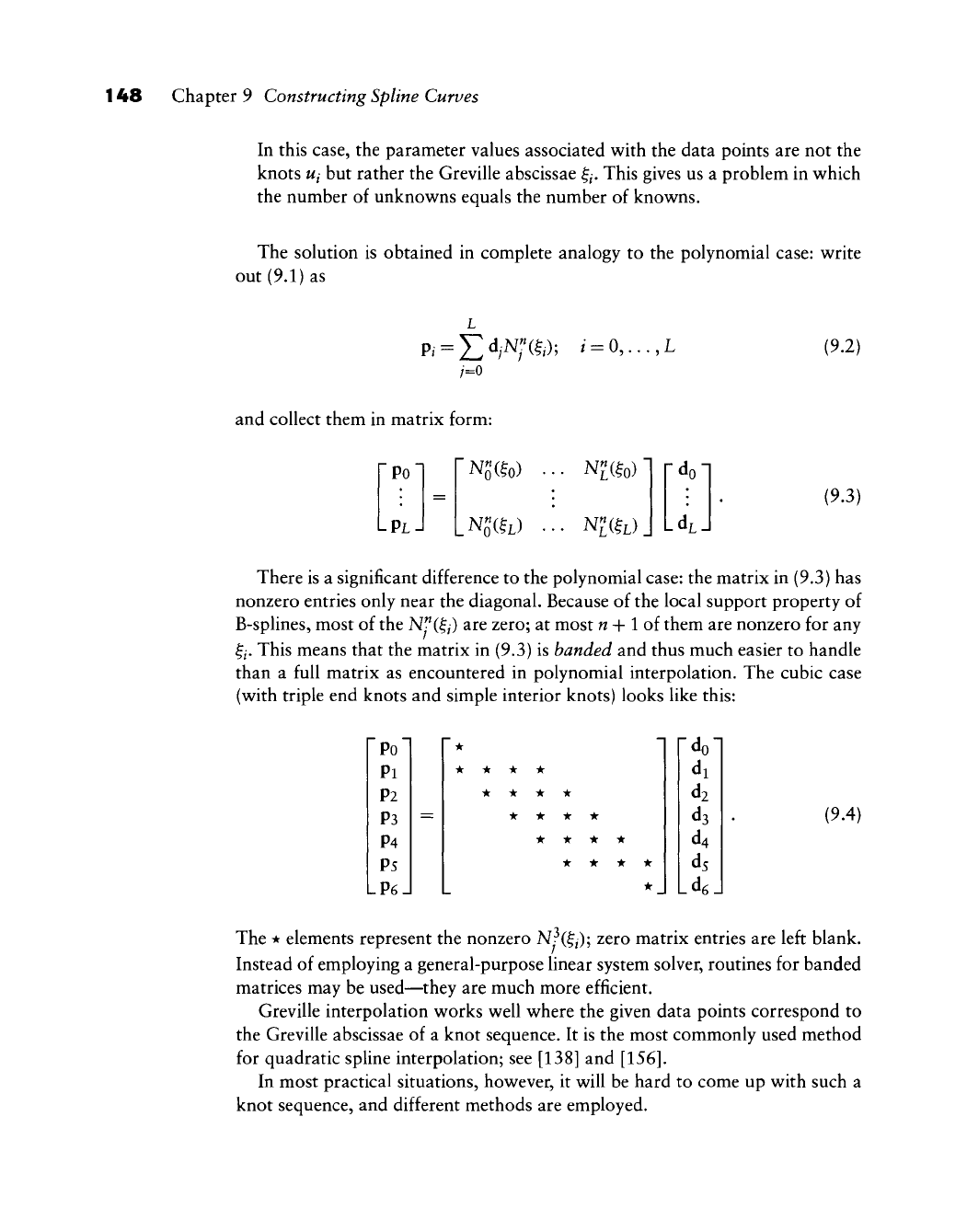
There is a significant difference to the polynomial case: the matrix in (9.3) has
nonzero entries only near the diagonal. Because of the local support property of
B-splines, most of the N^i^j) are zero; at most
w
+ 1 of them are nonzero for any
§^. This means that the matrix in (9.3) is banded and thus much easier to handle
than a full matrix as encountered in polynomial interpolation. The cubic case
(with triple end knots and simple interior knots) looks like this:
Po"
Pi
P2
P3
P4
P5
P6-
"•
* * * *
• * * •
• * * •
• * * *
* • * •
•
_
fdo
di
d2
ds
d4
ds
Ld6
(9.4)
The * elements represent the nonzero N^(§/); zero matrix entries are left blank.
Instead of employing a general-purpose linear system solver, routines for banded
matrices may be used—they are much more efficient.
Greville interpolation works well where the given data points correspond to
the Greville abscissae of a knot sequence. It is the most commonly used method
for quadratic spline interpolation; see [138] and
[156].
In most practical situations, however, it will be hard to come up with such a
knot sequence, and different methods are employed.
9.2 Least Squares Approximation 149
9.2 Least Squares Approximation
Curves are not always required to pass through a set of points; sometimes it may
suffice to be close to the given points. In this case, we speak of approximating
curves. We encountered situations Hke this in Section 7.8.
As an example, consider the generation of an airplane wing: its cross sections
(profiles) are defined by analytical means, optimizing some airflow characteristics
for example.^ One can now compute many (100, say) points on the profile and
then ask for a curve through them. A cubic spline interpolant would do the job,
but it would have too many segments—for a typical profile, a curve with 15
segments might provide a perfect fit. One possibility is to simply discard data
points until we are left with the desired number. We would then compute the
interpolant to the reduced data set and check if the discarded points are within
tolerance. This is expensive, and a more frequently encountered approach is one
that makes sure that all data points are as close as possible to the curve, avoiding
any iterations.
To make matters more precise, assume that we are given data points p^ with
/ = 0,. .., F? We wish to find an approximating B-spline curve p(w) of degree n
with K-\-\ knots
WQ?
• • • 5
^x- ^^ want the curve to be close to the data points
in the least squares sense. Suppose the data point p^ is associated with a data
parameter value Wi? Then we would like the distance ||p^
—
pCu^/)!!
to be small.
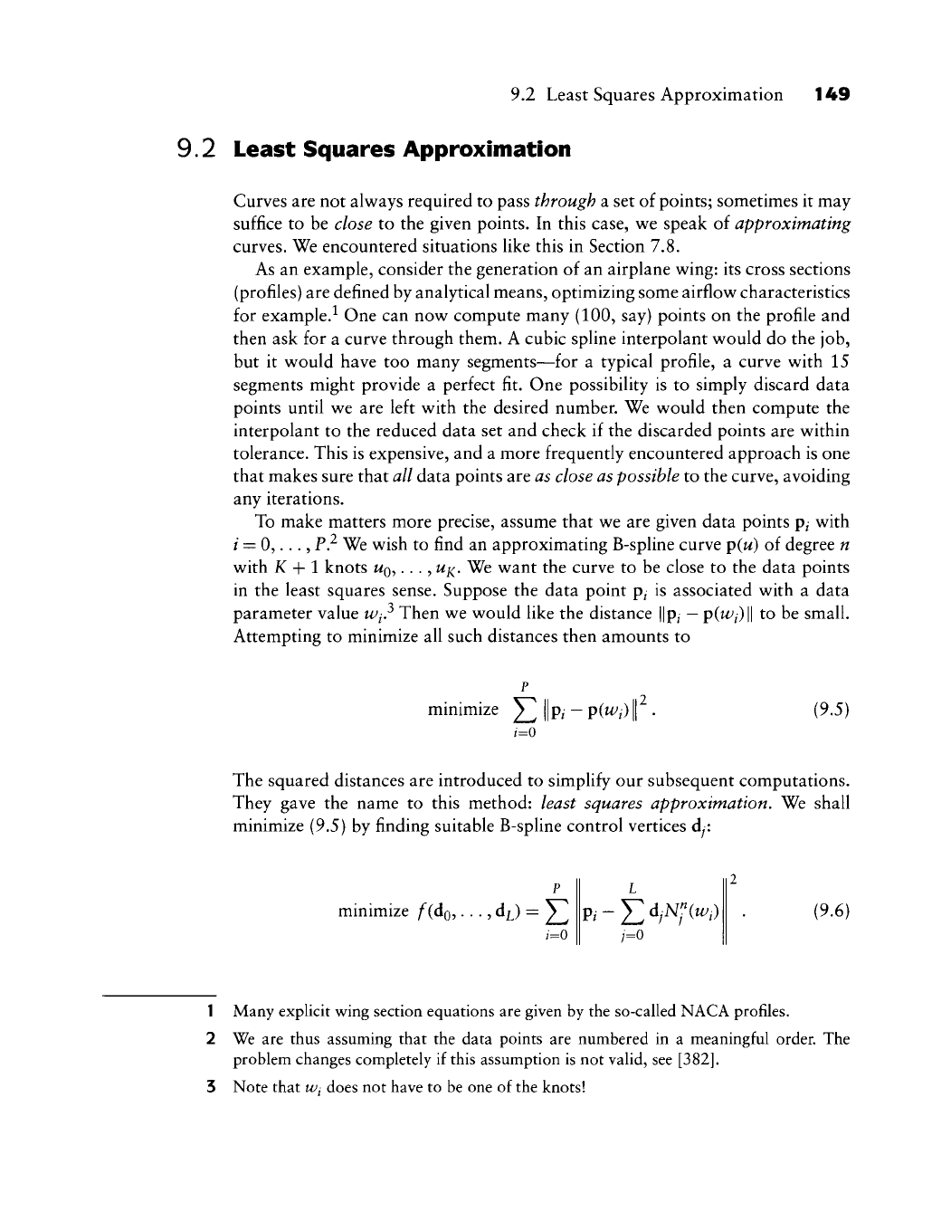
Attempting to minimize all such distances then amounts to
minimize Y^ ||p^
—
p(w//) |
(9.5)
The squared distances are introduced to simplify our subsequent computations.
They gave the name to this method: least squares approximation. We shall
minimize (9.5) by finding suitable B-spline control vertices dy:
minimize /^(do,..., d^^) = 2_.
p,-^d,N;(u/,) (9.6)
1 Many explicit wing section equations are given by the so-called NACA profiles.
2 We are thus assuming that the data points are numbered in a meaningful order. The
problem changes completely if this assumption is not valid, see
[382].
3 Note that
Wi
does not have to be one of the knots!
150 Chapter 9 Constructing Spline Curves
The least squares approach—identical to our development of the polynomial case
in Section 7.8—produces the normal equations
LP P
Y,
d;
J2
Nf(Wi)NliWi) =
J2 PtK(^i); fe = 0,...,
L.
(9.7)
This is a linear system of L + 1 equations for the unknowns d^, with a
coefficient matrix M whose elements my^^ are given by
p
The symmetric matrix M is often ill conditioned—special equation solvers,
such as a Cholesky decomposition, should be employed. For more details on the
numerical treatment of least squares problems, see
[376].
The matrix M is singular if and only if there is a span
[^y_i,
Uj_^^]
that contains
no Wj. This fact is known as the Schoenberg-Whitney theorem.
In cases where there are gaps in the data points, there is still a remedy: we may
employ smoothing equations in exactly the same way as was done in Section 7.9.
The addition of these equations, now applied to B-spline control vertices instead
of Bezier control vertices, will guarantee a solution. In cases where there is noise
in the data, these equations will also help in obtaining a better shape of the least
squares curve.
We have so far assumed much more than would be available in a practical
situation. First, what should the degree n ht} In most cases,
w
= 3 is a reasonable
choice. The knot sequence poses a more serious problem.
Recall that the data points are typically given without assigned data parameter
values Wi. The centripetal parametrization from Section 9.6 will give reasonable
estimates, provided that there is not too much noise in the data. But how many
knots
Uj
shall we use, and what values should they receive? A universal answer
to this question does not exist—it will invariably depend on the application at
hand. For example, if the data points come from a laser digitizer, there will be
vastly more data points p^ than knots w/.
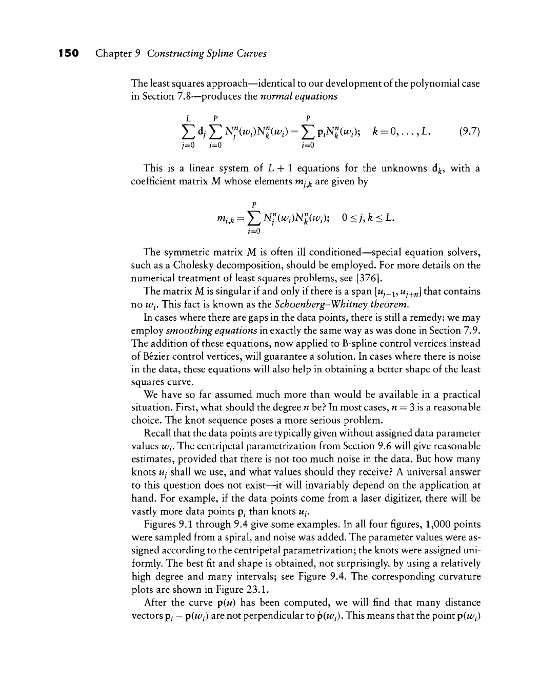
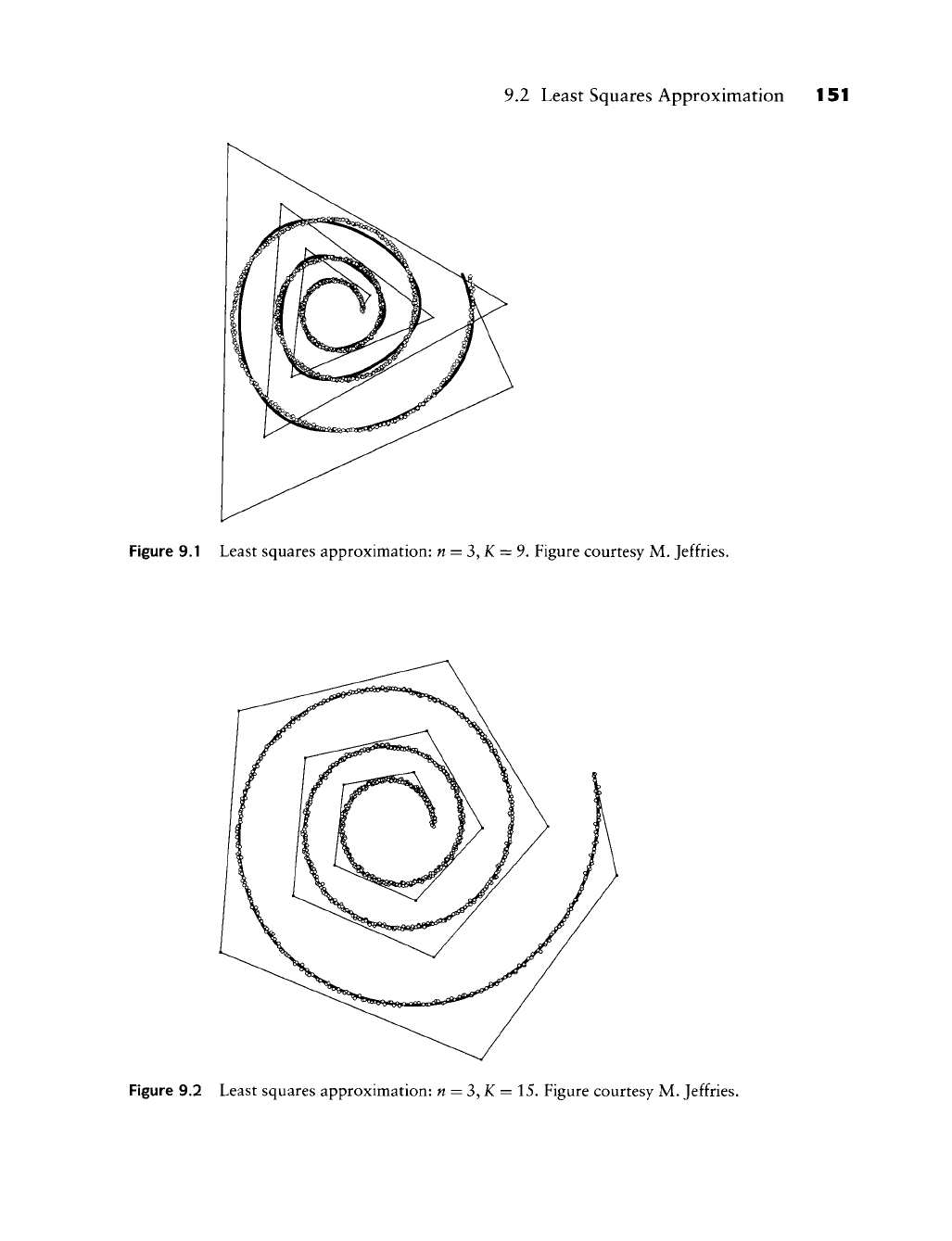
Figures 9.1 through 9.4 give some examples. In all four figures, 1,000 points
were sampled from a spiral, and noise was added. The parameter values were as-
signed according to the centripetal parametrization; the knots were assigned uni-
formly. The best fit and shape is obtained, not surprisingly, by using a relatively
high degree and many intervals; see Figure 9.4. The corresponding curvature
plots are shown in Figure 23.1.
After the curve p(w) has been computed, we will find that many distance
vectors
p^
—
p(w//) are not perpendicular to
p(w^/).
This means that the point p(w//)
9.2 Least Squares Approximation 151
Figure 9.1 Least squares approximation: n = 3,K = 9. Figure courtesy M. Jeffries.
Figure 9.2 Least squares approximation: n = 3,K = 15. Figure courtesy M. Jeffries.