Farin G. Curves and Surfaces for CAGD. A Practical Guide

Подождите немного. Документ загружается.

152 Chapter 9 Constructing Spline Curves

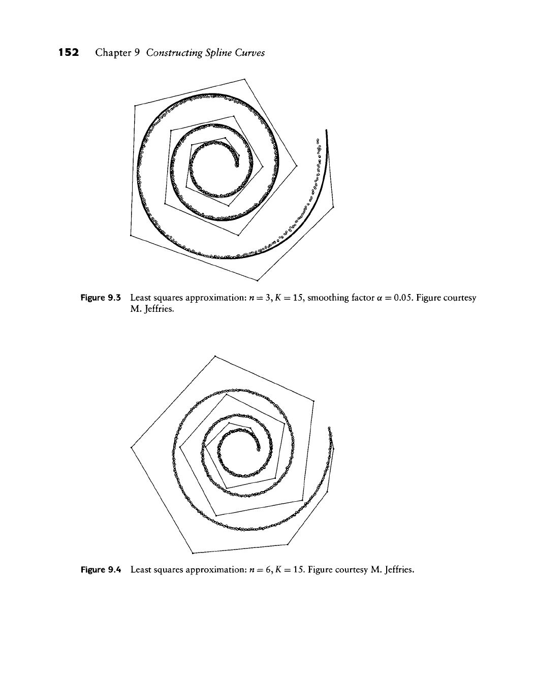
Figure 9.3 Least squares approximation:

= 3, K = 15, smoothing factor a = 0.05. Figure courtesy

M. Jeffries.

Figure 9.4 Least squares approximation: n = 6,K = 15. Figure courtesy M. Jeffries.

9.3 Modifying B-Spline Curves 153

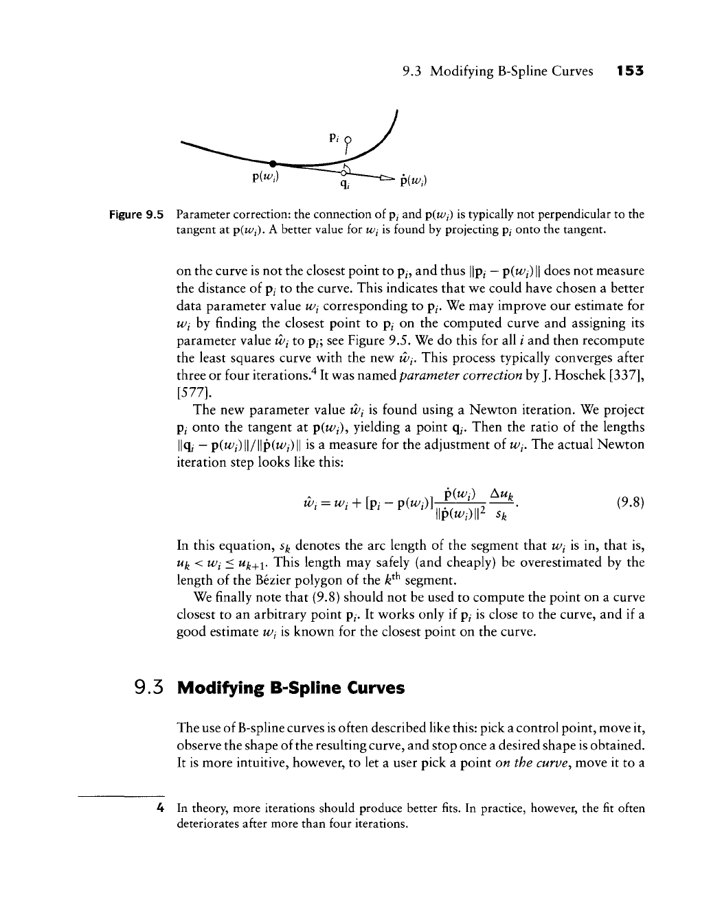
Figure 9.5 Parameter correction: the connection of

and piwj) is typically not perpendicular to the

tangent at

p(Wi).

A better value for

is found by projecting pi onto the tangent.

on the curve is not the closest point to

p^,

and thus ||p^

—

piWj)

does not measure

the distance of p/ to the curve. This indicates that we could have chosen a better

data parameter value Wj corresponding to p/. We may improve our estimate for

Wj by finding the closest point to p^ on the computed curve and assigning its

parameter value Wj to

p^;

see Figure 9.5. We do this for all / and then recompute

the least squares curve with the new Wj, This process typically converges after

three or four iterations."* It was named parameter correction by

Hoschek

[337],

[577].

The new parameter value Wi is found using a Newton iteration. We project

onto the tangent at p(u^^), yielding a point q^. Then the ratio of the lengths

llq^

—

p(t6'/)||/||p(t^^/)|| is a measure for the adjustment of

Wi,

The actual Newton

iteration step looks like this:

^. = "^. + [p.-pK)]^^^. (9.8)

llpKOIr sk

In this equation, s^ denotes the arc length of the segment that Wi is in, that is,

Uj^

< Wi <

Uj^^i.

This length may safely (and cheaply) be overestimated by the

length of the Bezier polygon of the k}^ segment.

We finally note that (9.8) should not be used to compute the point on a curve

closest to an arbitrary point p/. It works only if

is close to the curve, and if a

good estimate Wi is known for the closest point on the curve.

9.5 Modifying B-Spline Curves

The use of B-spline curves is often described like

this:

pick a control point, move it,

observe the shape of the resulting curve, and stop once a desired shape is obtained.

It is more intuitive, however, to let a user pick a point on the curve^ move it to a

4 In theory, more iterations should produce better fits. In practice, however, the fit often

deteriorates after more than four iterations.

154 Chapter 9 Constructing Spline Curves

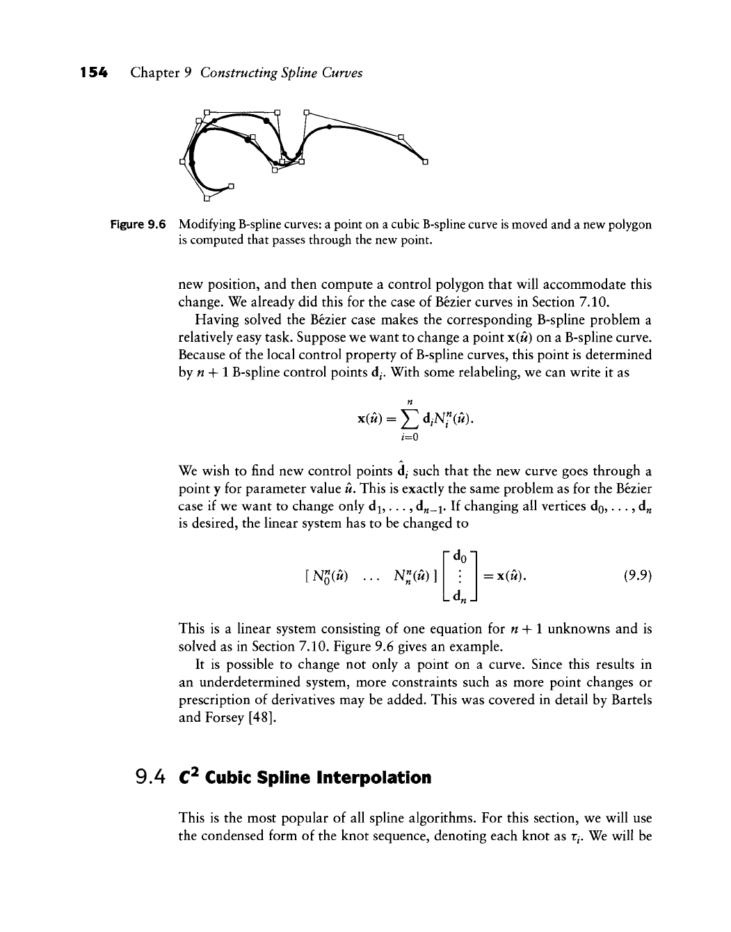
Figure 9.6 Modifying B-spline

curves:

a point on a cubic B-spline curve is moved and a new polygon

is computed that passes through the new point.

new position, and then compute a control polygon that will accommodate this

change. We already did this for the case of Bezier curves in Section 7.10.

Having solved the Bezier case makes the corresponding B-spline problem a

relatively easy task. Suppose we want to change a point x(u) on a B-spline curve.

Because of the local control property of B-spline curves, this point is determined

by n + 1 B-spline control points d^. With some relabeling, we can write it as

We wish to find new control points d^ such that the new curve goes through a

point y for parameter value u. This is exactly the same problem as for the Bezier

case if we want to change only

dj,...,

d„_i. If changing all vertices do,..., d„

is desired, the linear system has to be changed to

[N^(u)

N"„(u)

]

Ld„

= X(M). (9.9)

This is a linear system consisting of one equation for

+ 1 unknowns and is

solved as in Section 7.10. Figure 9.6 gives an example.

It is possible to change not only a point on a curve. Since this results in

an underdetermined system, more constraints such as more point changes or

prescription of derivatives may be added. This was covered in detail by Bartels

and Forsey [48].

9.4 C^ Cubic Spline Interpolation

This is the most popular of all spline algorithms. For this section, we will use

the condensed form of the knot sequence, denoting each knot as

Xj,

We will be

9.4 C^ Cubic Spline Interpolation 155

XQ X^ Xg

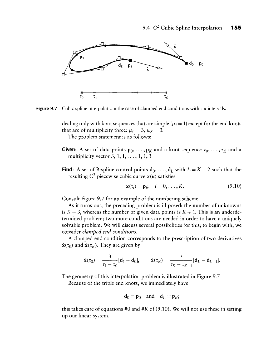
Figure 9.7 Cubic spline interpolation: the case of clamped end conditions with six intervals.

dealing only with knot sequences that are simple (/x^ = 1) except for the end knots

that are of multiplicity three:

/XQ

= 3,

/Xj^;

= 3.

The problem statement is as follows:

Given: A set of data points Po?

• • • ?

Px ^nd a knot sequence

TQ,

...,

T]^

and a

multiplicity vector 3,1,1,...,1,1,3.

Find: A set of B-spline control points do,..., d^^ with L = K -\-2 such that the

resulting C^ piecewise cubic curve x(u) satisfies

x(r,) =

p,-;

/ =

0,...,K.

(9.10)

Consult Figure 9.7 for an example of the numbering scheme.

As it turns out, the preceding problem is ill posed: the number of unknowns

is K + 3, whereas the number of given data points is K + 1. This is an underde-

termined problem; two more conditions are needed in order to have a uniquely

solvable problem. We will discuss several possibilities for this; to begin with, we

consider clamped end conditions,

A clamped end condition corresponds to the prescription of two derivatives

x(ro) and x(rx). They are given by

3 3

x(ro) = [di - do], xCr^) =

[d^^

d^-i].

Ti - to tx - Tj^-\

The geometry of this interpolation problem is illustrated in Figure 9.7

Because of the triple end knots, we immediately have

do = Po and di^ = px;

this takes care of equations #0 and #X of (9.10). We will not use these in setting

up our linear system.

156 Chapter 9 Constructing Spline Curves

The clamped end conditions yield

di = do + ^^^x(ro) and d,^_i = d^, - ^^^^^xCr^).

Thus,

the first and last equations of our linear system become

d2N|(ri) + daN^Cri) = r, and ^L-?>^1-2>^-^K-\) + ^L-l^l-ii^K-i) =

with

rs = Pi-diN^(ri) and r^ =

PK-1

- dL-iN^_i(rK-i).

Each of the remaining unknowns

d25...,

dj^_2 is related to the data points by

one equation. Because of the local support property of cubic B-splines, it is of

the form

= d,N3(r,) + d,+iN^i(r,) +

Ai^rn]^-^{x>);

i = 2,...,K-2. (9.11)

Together, these are iC

—

1 equations for the K

—

1 unknown control points. In

matrix form, we have

N|(T2)

Ni_3(rK_2) Ni_2(TK_2) H-l(-'K-2)

L^L-2

PK-2

L r^

(9.12)

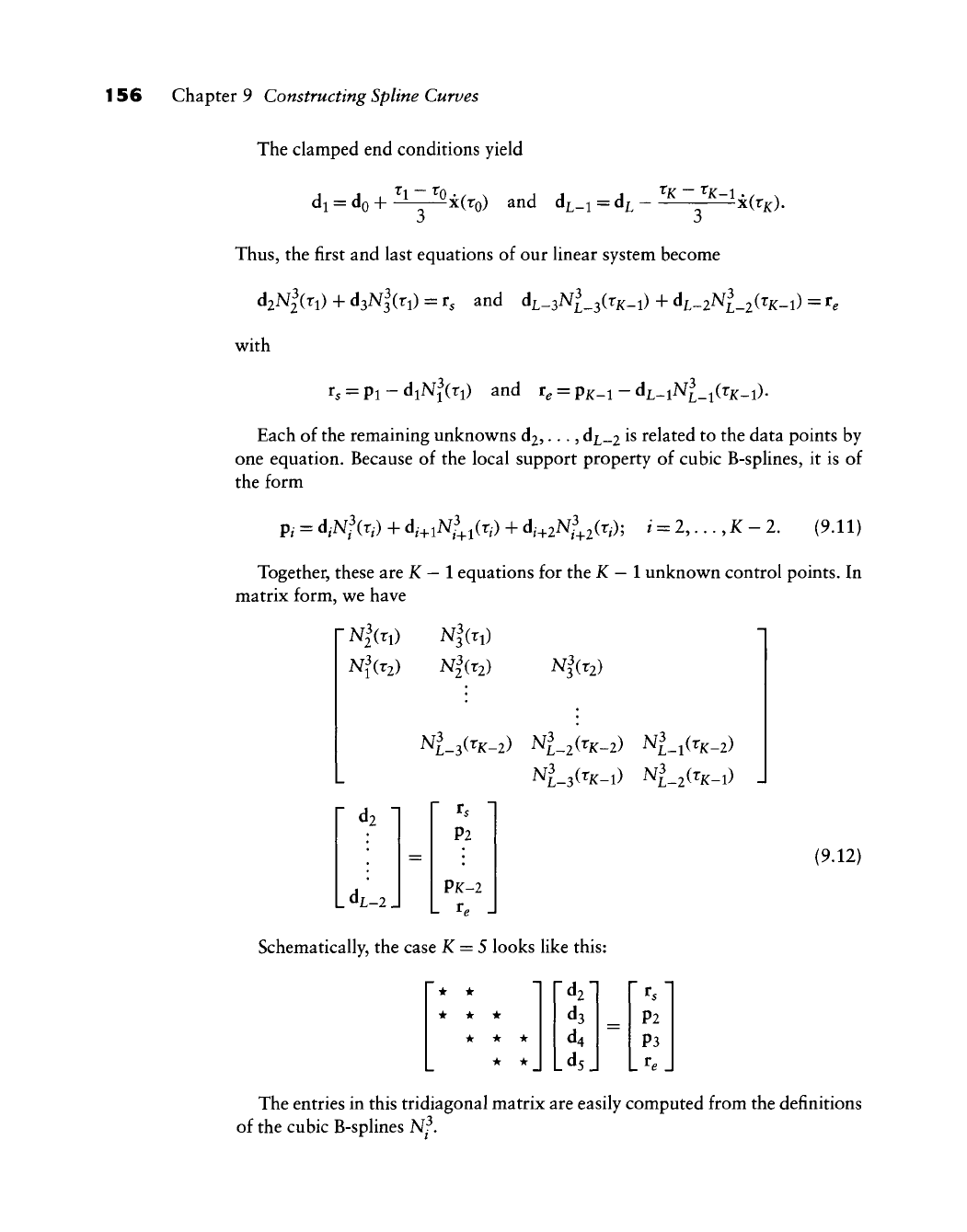
Schematically, the case K = 5 looks like this:

* •

• • •

• •

Ids]

.^e]

The entries in this tridiagonal matrix are easily computed from the definitions

of the cubic B-splines Nf,

9.5 More End Conditions 157

In the case of uniform knots

= /, the interpolation conditions (9.11) take

on a particularly simple form:

6p,-

= d, + 4d,+i + d,+2; / =

2,...,

X - 2. (9.13)

We conclude with a method for cubic spline interpolation that occasionally

appears in the literature (e.g., in Yamaguchi [621]). It is possible to solve the

interpolation problem without setting up a linear system! Just do the following:

define do, d^, dj^_i, d^^ as before, and set d/ = p/_i for all other control points.

Then, for / =

2,...,

—

2, correct the location of d^ such that the curve passes

through p^_i. Repeat until the solution is found.

This method will always converge and will not need many steps in order to

do so. So why bother with linear systems? The reason is that tridiagonal systems

are most effectively solved by a direct method, whereas the earlier iterative

method amounts to solving the system via Gauss-Seidel iteration. So though

geometrically appealing, the iterative method needs more computation time than

the direct method.

9.5 More End Conditions

For cubic spline interpolation, the choice of end conditions is important for the

shape of the interpolant near the endpoints—they do not matter much in the

interior. We have seen a clamped end condition earlier. It works well in situations

where the end derivatives are actually known. But in most applications, we do

not have this knowledge. Still, two extra equations are needed in addition to the

basic interpolation conditions (9.10).

We list several possibilities:

The natural end conditions are derived from the physical analogy of a wooden

beam that is clamped at some positions; see Figure 9.22. Beyond the first and last

clamps, such a beam assumes the shape of a straight line. A line is characterized

by having a zero second derivative, and hence the end conditions

x(ro) = 0, x(rx) = 0

are called natural end conditions.

The second derivative of a Bezier curve at bo is given by bo

—

2bi + b2. In

terms of B-spline control vertices (using triple end knots), this becomes

- 2di + -4^di + -4^d2 = 0,

AA+AI An + A,

158 Chapter 9 Constructing Spline Curves

where we set A^ = r^+i

—

r^ We rearrange and obtain

(Ao + Ai)do - (2Ao + Ai)di + Aod2 = 0. (9.14)

A similar condition holds at the other endpoint. Unless required by a specific

application, this end condition should be avoided since it forces the curve to

behave linearly near the endpoints.

Typically another end condition, called Bessel end condition, yields better

results. It works as follows: the first three data points and their parameter values

determine an interpolating quadratic curve. Its first derivative at po is taken to

be the one for the spline curve. If we set

a = — and

—

^2 -

"^0

and

lap

then

2 1

di=-(apo + ^a) + -po.

This value for dj is then used in the earlier clamped end condition. The control

point d£^_i is obtained in complete analogy; it is then also used for a clamped

end condition.

Other end conditions exist: requiring x(ro) = x(ri) is called a quadratic end

condition. If all data points and parameter values were read off from a quadratic

curve, then this condition would ensure that the spline interpolant reproduces

that quadratic. The same is true, of course, for the Bessel end conditions. If

the first and second cubic segment are parts of one cubic, then their third

derivatives at X\ would agree. The corresponding end condition is called not-

a-knot condition since the knot r^ does not act as a breakpoint between two

distinct cubic segments.

We finish this section with a few examples, courtesy T. Foley, using uni-

form parameter values in all examples.^ Figure 9.8 shows equally spaced data

5 Owing to the symmetry inherent in the data points, all parametrizations discussed later

yield the same knot spacing. All circle plots are scaled down in the }/-direction.

9.5 More End Conditions

159

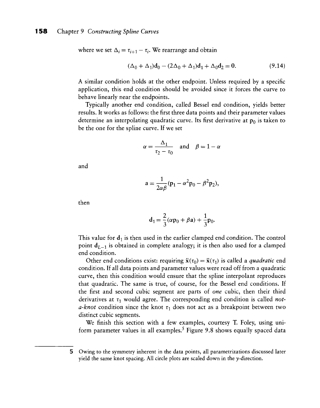
Figure 9.8 Exact clamped end condition spline.

K=l

K=0

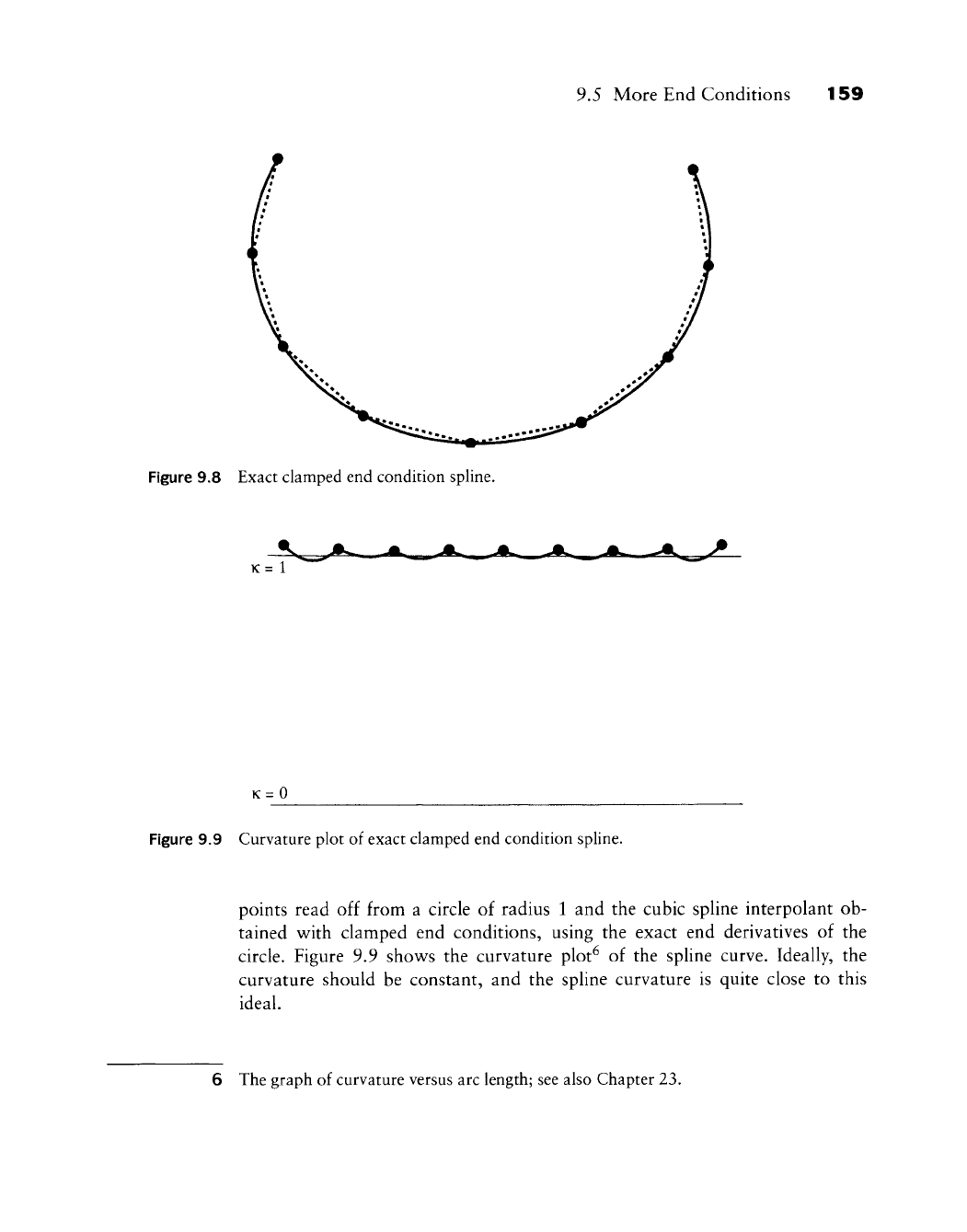
Figure 9.9 Curvature plot of exact clamped end condition spline.

points read off from a circle of radius 1 and the cubic spline interpolant ob-

tained with clamped end conditions, using the exact end derivatives of the

circle. Figure 9.9 show^s the curvature plot^ of the spline curve. Ideally, the

curvature should be constant, and the spline curvature is quite close to this

ideal.

6 The graph of curvature versus arc length; see also Chapter 23.

160 Chapter 9 Constructing Spline Curves

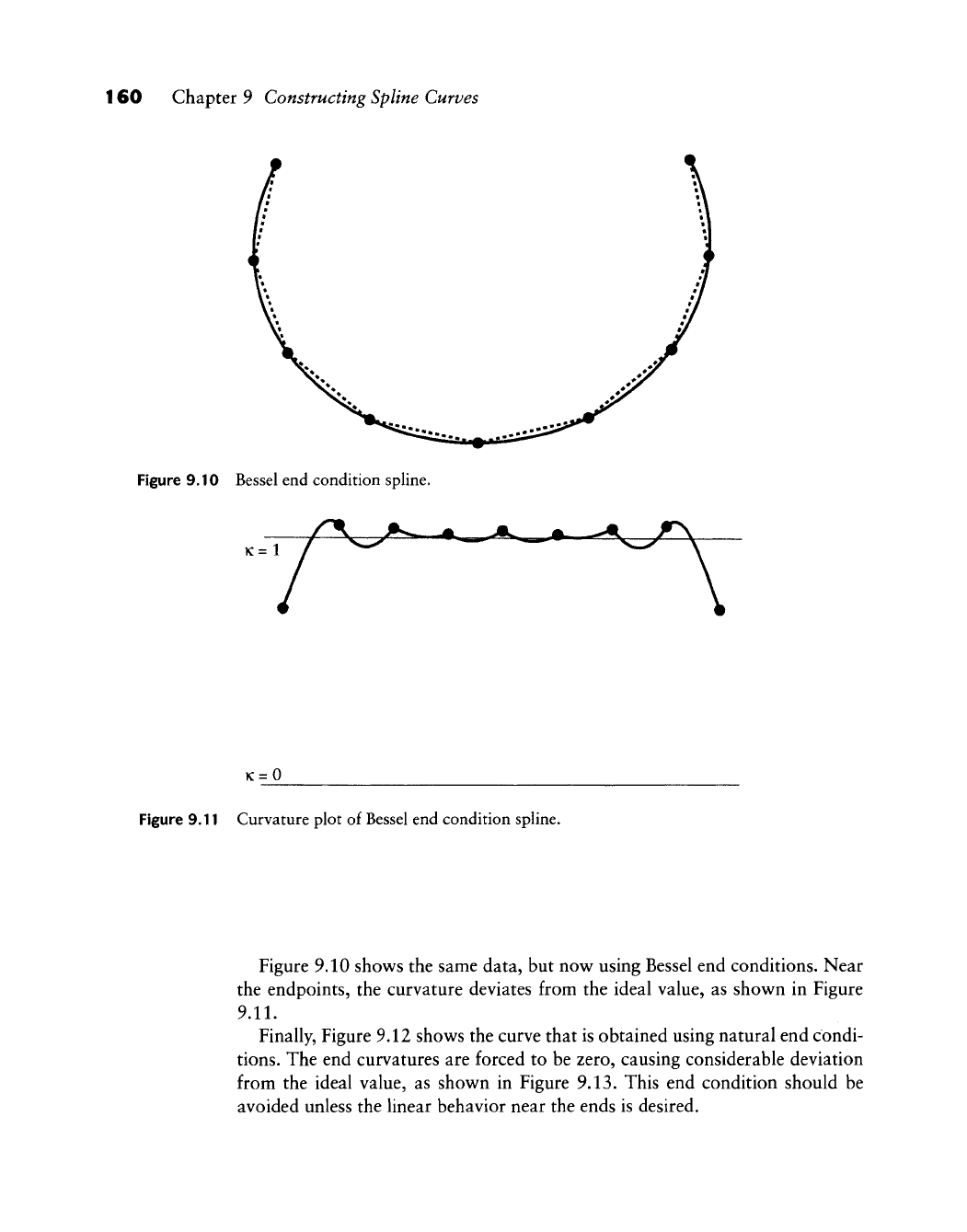
Figure 9.10 Bessel end condition spline.

K=l

K=0

Figure 9.11 Curvature plot of Bessel end condition spline.

Figure 9.10 shows the same data, but now using Bessel end conditions. Near

the endpoints, the curvature deviates from the ideal value, as shown in Figure

9.11.

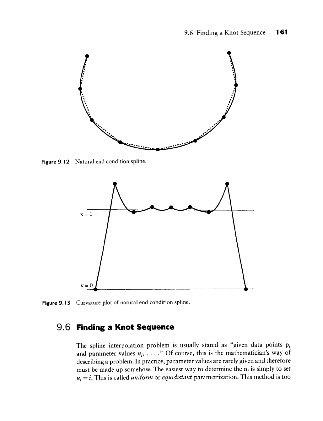
Finally, Figure 9.12 shows the curve that is obtained using natural end condi-

tions.

The end curvatures are forced to be zero, causing considerable deviation

from the ideal value, as shown in Figure 9.13. This end condition should be

avoided unless the linear behavior near the ends is desired.

9.6 Finding a Knot Sequence 161

Figure 9.12 Natural end condition spline.

K=l

K=0

Figure 9.13 Curvature plot of natural end condition spline.

9.6 Finding a Knot Sequence

The spline interpolation problem is usually stated as "given data points p^

and parameter values w^, . ..." Of course, this is the mathematician's way of

describing a problem. In practice, parameter values are rarely given and therefore

must be made up somehow. The easiest way to determine the ui is simply to set

= i. This is called uniform or equidistant parametrization. This method is too