Feny? D. (Ed.) Computational Biology

Подождите немного. Документ загружается.

161

3-D Structures of Macromolecules Using Single-Particle Analysis in EMAN

focus that internal detail in the particles, or the shape of the

particles is obscured. Images with either poor contrast or

those too far from focus should be discarded.

5. Next, the “FFT” box in the control panel can be checked.

This will display the power spectrum of the image. A detailed

discussion of the interpretation of such power spectra is beyond

this manuscript, but certain asymmetries in the power spec-

trum can indicate astigmatism or drift and indicate images,

which should be discarded. Though not used here the program

ctﬁt can also be useful in this process.

1. The image assessment process will typically eliminate any-

where from one to three quarters of the raw micrographs. The

next step is to locate particles within each image.

2. In the initial steps only a few of the best micrographs are

used, with the goal of initially picking 1,000–2,000 high con-

trast particles. At this stage it may not be entirely clear what is

and is not a particle in the images, and anything which may

be a particle should be selected. This will be resolved in

Subheading 3.4, after which Subheading 3.3 is revisited for

improved particle picking.

3. Prior to selecting particles, the raw images should be normal-

ized. That is, the mean and standard deviation of the images

should be adjusted, and optionally the contrast may be

inverted. For each image : “proc2d <imageﬁle> <imageﬁle>

edgenorm inplace [invert] ”. If the images are in .DM3 format

(see Note 15), the second ﬁlename should be replaced with

the “.mrc” extension, and the “image.mrc” ﬁle should be

used in the next step. The invert option should be speciﬁed if

3.3. Particle Picking

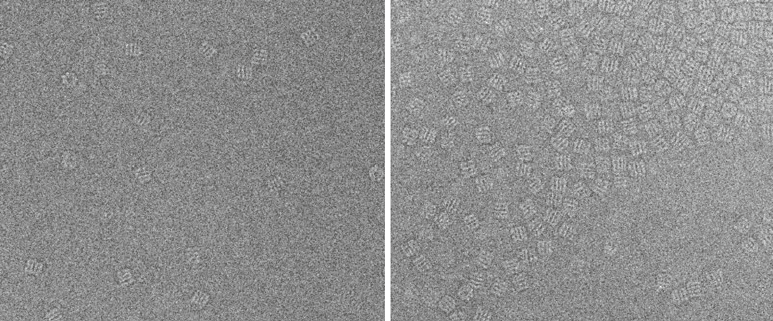
Fig. 1. GroEL in vitreous ice. Both of these images exhibit good contrast, but the left image is properly monodisperse,

whereas the image on the right exhibits much too high a concentration and would not be processed.

162 Ludtke

your particles appear dark on a white background. If the

particles appear white on a dark background, they do not

require inversion. For images that are too oversampled, the

shrink=<n> option may be used to reduce the sampling by an

integral factor of <n>, and increase Å/pix by the same

factor.

4. Executing “boxer <imageﬁle>” will cause three windows to

open (see Note 7). One window is the control panel with

various input ﬁelds and a menu, the second contains the

micrograph, and the third will initially be empty. This pro-

gram must be run once for each micrograph to be boxed.

5. In general the box size should be about 1.5× larger than your

particles. “Measure” in the control panel, can be used to esti-

mate the size of your particle in pixels by left-dragging in the

image window. The longest axis of a representative particle

should be measured, then multiplied by 1.5, and ﬁnally

rounded down to a “good” size. “Good” box sizes are those

with prime factors less than 11 and divisible by 8. “Good”

sizes include the following: 40, 48, 64, 80, 96, 112, 128,

144, 160, 192, 256. Once determined, the size should be

entered in the boxer control panel, and the same size used

thereafter for each micrograph.

6. Particles must now be selected from the image. The image

can be panned by right-dragging on the image, or using the

panning widget in the control panel. The zoom factor can be

adjusted in the boxer control panel. Particles may be selected

either manually or semiautomatically at this point. For man-

ual picking, “Select” should be toggled in the control panel,

then individual particles must be manually clicked on in the

micrograph view. Each particle will appear in the third win-

dow as it is selected. Left-dragging can be used to properly

center each particle. Bad particles can be deleted using the

“Delete” mode in the boxer control panel.

7. For semi-automatic selection, which should be followed by

manual pruning, 3–5 particles should be selected manually,

then “Autobox” from the “Boxes” menu in the control panel

can be used. This will cause a window with four sliders to

appear, and some additional particles to be automatically

selected. At this point the magniﬁcation of the image should

be reduced so the entire micrograph is visible in the image

display. The automatically picked particles are conﬁned to a

region adjacent to the ﬁrst selected reference. As the sliders

are adjusted, it will update the automatically picked particles

in this region. The ﬁrst slider is used to decide how closely the

potential particles must match the references. The second

and third sliders are used to exclude potential particles whose

163

3-D Structures of Macromolecules Using Single-Particle Analysis in EMAN

contrast is too high or too low. Once the sliders have been

adjusted for the preview region, “OK” will trigger autoselec-

tion of the entire micrograph.

8. This process should continue until a total of ~1,000 particles

have been selected from the set of best micrographs. After

each micrograph is complete “Save Boxed Particles” and

“Save Box DB” must be selected from the “Boxes” menu.

The default ﬁlenames are appropriate for both ﬁles. Boxer can

then be exited and restarted for the next micrograph.

1. To proceed with 2-D analysis the boxed-out particles from

the individual images must be combined into a single-particle

stack ﬁle. This is best done in a subdirectory to avoid having

too many output ﬁles in one place. Type “mkdir r2d; cd r2d”.

The most efﬁcient method for producing a usable stack ﬁle is

to type “lstcat.py all.lst ../*.hed” where “../*.hed” will refer-

ence all of the boxed-out particle ﬁles you saved in the previ-

ous step. This should be followed by “lstfast.py all.lst”. These

operations produce a text ﬁle “all.lst” which EMAN will treat

as an image ﬁle containing all of the particles you have

selected.

2. Filtering and/or further downsampling the particle data is

recommended for this preliminary analysis. This may produce

improved results in addition to speeding the process. The fol-

lowing command will perform a low-pass ﬁlter and down-

sample by a factor of 2: “proc2d all.lst start.hed apix=<A/pix>

lp=20 shrink=2 edgenorm”.

3. Next, the program reﬁne2d.py must be applied to the particle

stack. Execute “reﬁne2d.py all.lst –iter=8 --ninitcls=50”. For

those with multi-core workstations, “--proc=<ncores>” may be

appended to the command for more speed.

4. A number of ﬁles will be produced by this command. The ﬁle

containing the ﬁnal results is called “iter.ﬁnal.img” (see

Note 15).

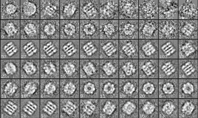
5. Display iter.ﬁnal.img either with the eman browser or by

running “v2 iter.ﬁnal.img” (Fig. 2). Class-averages should

represent a variety of different views of the particle under

study (see Notes 8 and 9). Class-averages representing con-

tamination, or other undesirable images may also appear.

6. Now that a better idea of what is present in the images has

been obtained, the next step is to return to 3.3 and complete

the particle selection process for all of the micrographs (see

Note 10). If there are a signiﬁcant number of “bad” class-

averages, it is best to also reselect the particles from the micro-

graphs already completed, being more conservative in the

selection process. If reboxing is performed, be sure to remove

3.4. 2-D Analysis

164 Ludtke

existing .hed and .img files before beginning. For the

low-resolution reconstruction outlined here, 2,000–3,000

particles in total should be more than sufﬁcient (perhaps as

many as 5,000 for asymmetric objects).

1. There are several methods for producing an initial model

which will reﬁne to an accurate structure. There is also con-

siderable controversy in the community over how good an

initial model needs to be. In EMAN, we believe even abstract

shapes or random patterns will have a strong propensity to

reﬁne to the correct structure. However for each particle,

there will be a small number of “local minima,” incorrect

structures which the reﬁnement process may “stick” at if

obtained. Rather than resort to difﬁcult experimental meth-

ods such as random conical tilt, we take the approach of

simply reﬁning several random starting models, and assessing

the ﬁnal results of each reﬁnement. Generally one or more of

the reﬁnements will lead to the correct solution (see Notes

11 and 17).

2. makeinitialmodel.py can be used to produce a manually speci-

ﬁed or randomly generated initial model. Simply executing the

3.5. Initial Model

Determination

Fig. 2. Class-averages produced from a set of 838 GroEL particles. The number in the corner of each class-average

indicates how many particles the average was constructed from. Note that most of the very poor images or images with

contamination came from a small number of particles. Also note that GroEL exhibits a fairly strongly preferred orientation,

showing many of the characteristic rectangular side views and many of the sevenfold symmetric top views, but very few

orientations in between. While this is not optimal, the wide range of different side views is sufﬁcient to obtain an unam-

biguous 3-D reconstruction.

165

3-D Structures of Macromolecules Using Single-Particle Analysis in EMAN

program will prompt for the necessary information. The starting

model must use the same box size as the particle data, and in

general should be approximately the same size as the particle.

From the class-averages in Subheading 3.4, it may be fairly

obvious what shape the particle has, and one reasonable start-

ing model would be something vaguely similar to this shape.

A random model is also quite acceptable (see Note 12).

3. If a structure has or may have symmetry, “proc3d model.mrc

model.mrc sym=<sym spec>” will impose it. “<sym spec>” may

be one of c<n>, d <n>, icos, tet or oct, for example, “sym=d7”

could be used for GroEL at low resolution. (see Note 13).

4. The resulting starting model will be written to model.mrc.

The model can be visualized in projection using “v4 model.

mrc” or in isosurface display using UCSF Chimera (http://

www.cgl.ucsf.edu/chimera/) or in EMAN2 using “e2display.

py model.mrc”.

5. It is best to run reﬁnements in a subdirectory as with 2-D

reﬁnement: “mkdir initial1; cd initial1”. The starting model

must be called threed.0a.mrc, but again, we would like to

reduce the size for speed at this point so: “proc3d ../model.

mrc threed.0a.mrc meanshrink=2”.

6. The particles must also be copied into this directory and

reduced: “lstcat.py all.lst ../*.hed” followed by “proc2d all.lst

start.hed shrink=2 apix=<A/pix> lp=20 edgenorm”.

7. Now a reﬁnement can be run: “reﬁne 8 mask=<boxsize/4>

hard=35 ang=7.5 pad=<see below> classkeep=1 classiter=5

xﬁles=<A/pix x2>,<mass in kDa>,99 phasecls [sym=<sym spec>]

[proc=<maxproc>]”. “pad=” should be set to the original box

size*3/4 rounded to the nearest “good” size. “mask=”

should be the original box size/4. If there is no symmetry,

“ang=” may be increased to 9 for speed. For very high sym-

metries such as icosahedral ang= may be reduced to 5. This

process may take some time to run depending on the sym-

metry, box size, and speed of your processor.

8. When the reﬁnement is complete there will be a large number

of different ﬁles in the directory. The primary ﬁles of interest

are “threed.?a.mrc” and “classes.?.img”.

9. As a ﬁrst step in assessing the reﬁnement results, “v4 threed.?a.

mrc” will open one window for each iteration of the recon-

struction process, which can be rotated together. The last

window will represent threed.8a.mrc, and contains the ﬁnal

results of the reﬁnement run. Ideally, there will be little dif-

ference between threed.7a.mrc and threed.8a.mrc. If there

are still signiﬁcant changes from one iteration to the next you

may consider running additional iterations of reﬁnement.

Running the same “reﬁne” command, but replacing “8” with

166 Ludtke

“12” will continue the refinement process through 12

iterations (for example).

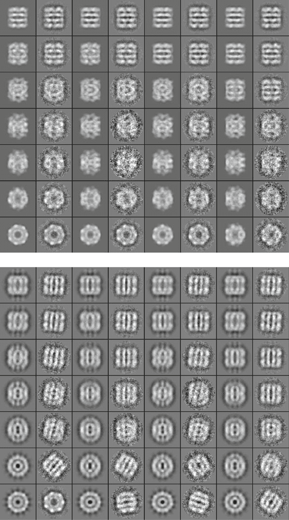
10. The next step is to assess the self-consistency of the recon-

struction using the eman browser or v2 to look at classes.8.img

(Fig. 3). This ﬁle contains pairs of projections of the 3-D

model and class-averages generated from the particles. Ideally

each adjacent pair of images should be identical, although the

second image will inevitably be noisier, as less averaging has

been performed. Some orientations may have few particles,

meaning these averages will be quite noisy and may not look

much like the corresponding projection. This is harmless, as

such averages are excluded from the reconstruction. However,

if there are several projections with strong averages which

match the projection poorly, this is an indication of an incor-

rect model.

11. Regardless of whether an apparently good starting model

was produced, this process, starting at step 2 should be

repeated multiple times (using a new directory, initial# for

each try). After several tries, the results should be assessed.

Ideally, more than one of the reﬁnements will have produced

basically the same, clearly accurate, structure. If no clearly

correct result has been obtained, the process may be contin-

ued additional times. If a self-consistent result still cannot

be obtained, there is a possibility that the data contains

structural heterogeneity, and cannot form a single self-con-

sistent structure. In this situation other methods may be

considered (7–9). Alternatively, contacting the EMAN

developers may be worthwhile.

1. Once a reliable initial model has been obtained, a full recon-

struction can be completed. This is virtually identical to the

reﬁnement process in Subheading 3.5, except the fully sam-

pled data is used, and thus the reﬁnements will be more time

consuming.

2. A suitable empty subdirectory should, once again, be created

“mkdir reﬁne1; cd reﬁne1”, and the particle data prepared:

“lstcat.py start.lst ../*.hed; lstfast.py start.lst”. Once again, the

data should be low-pass ﬁltered to roughly the ﬁrst zero of

the CTF, which we will assume is at ~20 Å: “proc2d start.lst

start.hed apix=<A/pix> lp=20”.

3. Next, copy threed.8a.mrc from whichever directory con-

tained the best model to be the starting model for this reﬁne-

ment, also returning it to the original box size: “proc3d ../

initial3/threed.8a.mrc threed.0a.mrc scale=2.0 clip=<boxsize>,

<boxsize>,<boxsize>”, replacing initial3 with the correct directory.

<boxsize> is the original, unreduced box size in pixels.

3.6. Reﬁnement

167

3-D Structures of Macromolecules Using Single-Particle Analysis in EMAN

Fig. 3. Comparison of projections and class-averages for a correct top and an incorrect bottom reconstruction. Note

that in the top set, there is excellent agreement between each horizontal pair of images. In the bottom set, while

many of the pairs match well, many also do not. Due to the iterative reﬁnement strategy, some of the projections and

averages will always agree, but for a structure to be correct, all of the high contrast averages should agree with their

projections.

168 Ludtke

4. Finally, we are ready to run the reﬁnement: “reﬁne

8 mask=<boxsize/2> hard=25 ang=<ang> pad=<as above x2>

classkeep=1 classiter=3 xﬁles=<A/pix>,<mass in kDa>,99 phasecls

[sym=<sym spec>] [proc=<maxproc>]”. This is very much like

the reﬁnement above, except our box size is now twice as

large. “ang=” may also be reduced somewhat to produce ﬁner

angular sampling and thus more projections. Since CTF cor-

rection still is not being performed, “ang=5” is probably suf-

ﬁcient. “classiter=” has also been reduced from 5 to 3, which

provides less protection from model bias (16), but will pro-

duce higher resolution reconstructions. There are many other

documented options which may be added for potentially

improved results, such as “amask=”, “useﬁlt”, and “fscls”.

5. Once the reﬁnement is complete (this will take as much as

~10–20× longer than the earlier reﬁnement), in addition to

examining the output ﬁles as above, the resolution of the

model should be evaluated. This process is only marginally

useful without CTF correction, but should still be completed.

The standard resolution assessment method in single-particle

analysis is to split the particle data into even and odd halves,

and do a 3-D reconstruction for each half, then compare them

with a Fourier shell correlation (FSC) function. To produce

the two reconstructions: “eotest mask=<boxsize/2> hard=25

pad=<as above x2> classkeep=1 classiter=3 xﬁles=<A/pix>,<mass

in kDa>,99 phasecls [sym=<sym spec>] [proc=<maxproc>]”. The

options are a subset of the options used for reﬁne, though this

command will take only a short time to complete.

6. To perform the FSC comparison, execute the eman browser

and select “Convergence” from the “Analysis” menu. This

will run some computations, then prompt for an Å/pixel

value. After providing this, a plot will appear. This plot will

contain one dark line and a number of thinner, lighter lines.

The dark line represents the FSC resolution test.

7. Ideally, this FSC curve will begin (low resolution) at 1.0, at

some resolution it will begin falling toward zero, and it will

oscillate randomly around zero until the end of the curve

(high resolution). In some cases, the curve will fall, but will

not reach zero, and may even move higher again. This can be

caused by either insufﬁcient sampling (ang=too large), aggres-

sive masking (primarily if the amask=option is used aggressively

in reﬁnement or if the box size is too small) or other arti-

facts. If the curve falls to zero, then the resolution can be

estimated as the point at which the FSC falls below 0.5 (see

Note 14).

8. The other thinner curves in this plot are not an indication of

resolution, but rather of convergence. These curves compare

each iteration with the previous iteration in the reﬁnement

169

3-D Structures of Macromolecules Using Single-Particle Analysis in EMAN

process. As the reﬁnement progresses, these lines should

gradually move to higher resolution (right) and higher FSC

scores (up). When convergence has been reached, from one

iteration to the next, the curves will remain basically the same.

If convergence has not been reached, additional reﬁnement

iterations (step 4) should be executed by increasing the

parameter 8 immediately after the “reﬁne” command.

9. The ﬁnal reconstruction is the highest numbered threed.?a.

mrc ﬁle.

Note that we have sidestepped the process of CTF correction

which is required to achieve a high resolution reconstruction.

In addition, this structure will lack CTF amplitude correction,

meaning there will be some subtle localized distortions even at

low resolution. However, this protocol should have at least

produced a low-resolution structure with the correct overall shape,

and make a suitable starting point for future CTF corrected recon-

structions. The more complicated protocols for CTF corrected

reconstruction, running on clusters and handling large numbers

of particles are discussed in the built-in tutorial in eman,

the workﬂow interface in EMAN2 and in earlier publications

(10, 17, 18).

1. As of this writing, EMAN is undergoing a major transition

from EMAN1 to EMAN2 (11). While EMAN2 will eventu-

ally obsolete EMAN1, and it contains a workﬂow interface

which dramatically simpliﬁes the reconstruction process, it is

currently still in development. The overall reconstruction

strategy described here for EMAN1 will largely still apply in

EMAN2. Notes have been added where signiﬁcant differ-

ences exist, or where EMAN2 may be more suitable. It is

completely safe to install EMAN2 within the same user

account as EMAN1. All EMAN2 programs begin with the

preﬁx “e2” to avoid naming conﬂicts between EMAN1 and

EMAN2.

2. It can be difﬁcult to optimize experimental conditions to pro-

duce the necessary monodisperse particles with good contrast.

Many routinely used buffer components have a substantial

negative impact on image contrast in cryo-EM experiments.

The most important of these is glycerol. The presence of

even a small percentage of glycerol can dramatically reduce

imaging contrast, and should be eliminated, if at all possible.

Detergent, added to stabilize membrane proteins, can also

4. Notes

170 Ludtke

cause substantial difﬁculties, and while clearly it cannot be

eliminated, reducing its concentration as much as possible

without making your particles unstable is an important

step. Detergent at concentrations above CMC will produce

micelles, which may be visible in the images, and can be

confused with the target particles in some situations. The key

to remember is that anything present in the specimen will

appear in the electron micrographs regardless of whether it is

biochemically inert.

3. One common approach for difﬁcult specimens is to use a con-

tinuous carbon substrate, but it is important to be aware that

this carbon will add to the noise level of the images, and fre-

quently leads to a preferred particle orientation, which in some

cases can make a reliable 3-D reconstruction impossible.

4. If you are experiencing problems with preferred particle ori-

entations in the absence of a continuous carbon substrate,

one possible solution is to add a very low concentration (well

below CMC) of detergent, which may help prevent hydro-

phobic patches on the particles from sticking to the surface of

the buffer.

5. In EMAN2, the main GUI programs are e2desktop.py, e2work-

ﬂow.py, e2boxer.py, e2ctf.py, and e2display.py.

6. In the future, the program e2workﬂow.py in EMAN2 will take

you step by step through the reconstruction process includ-

ing CTF correction, but as of this writing it is not yet com-

plete, and cannot yet be run on linux clusters.

7. The EMAN2 program e2boxer.py can perform interactive

semiautomatic particle picking on several micrographs at

once, and is a good an alternative to boxer. A number of excel-

lent non-EMAN particle pickers also exist (19). The proc2d

command can be used for ﬁle format conversion even if a

non-EMAN particle picker is used.

8. Reference free class-averages should be closely examined for

signs of signiﬁcant dynamics in the particle. If several class-

averages seem to be in the same orientation, but one domain

is undergoing substantial motion, this may be a sign of a

structurally heterogeneous particle. If the motion is relatively

small and localized, 3-D reconstruction may still be possible

using the method presented here. For larger motions or other

forms of heterogeneity, see (7–9).

9. Preferred orientation can be a signiﬁcant problem. If the

class-averages seem to largely represent a single view of the

specimen, it may be impossible to achieve an accurate 3-D

reconstruction. While it is not necessary to have all possible

orientations, the minimum requirement for a complete 3-D

reconstruction is to have particles covering at least one