Gao R.X., Yan R. Wavelets: Theory and Applications for Manufacturing

Подождите немного. Документ загружается.

transform and other commonly used techniques, in terms of the choice of the

template functions fc

ðtÞg

n2z

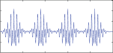
. To illustrate the p oint, a nonstationary signal

as shown in Fig. 2.1 is used as an example. The signal consists of four groups

of impulsive signal trains, each containing two transient elements of different

center frequencies at 1,500 and 650 Hz, respectively. The four groups are separated

from one another by a 12-ms time interval. Within each group, the two transient

elements are time-overlapped. The sampling frequency used to captu re the signal

is 10 kHz.

2.1 Fourier Transform

The Fourier transform is probably the most widely applied signal processing tool

in science and engineering. It reve als the frequency composition of a time series

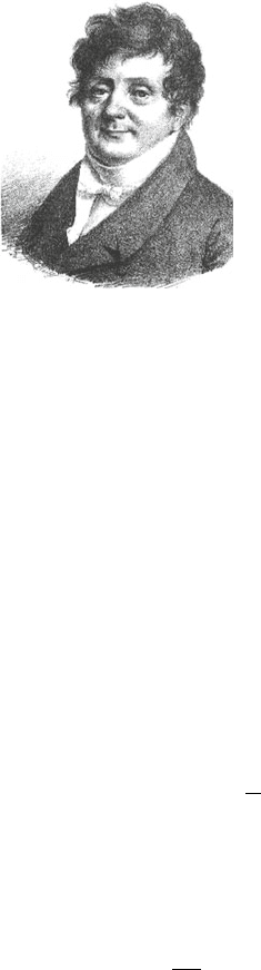
xðtÞ by transforming it from the time domain into the frequency domain. In 1807,

the French mathematician Joseph Fourier (Fig. 2.2) found that any periodic signal

can be presented by a weighted sum of a series of sine and cosine functions.

However, because of the uncompromising objections from some of his contempor-

aries such as J. L. Lagrange (Herivel 1975), his paper on this ﬁnding never

got published, until some 15 years later, when Fourier wrote his own book, The

Analytical Theory of Heat (Fourier 1822). In that book, Fourier extended his

ﬁnding to aperiodic signals, stating that an aperiodic signal can be represented by

a weighted integral of a series of sine and cosine functions. Such an integral is

termed the Fourier transform.

Using the notation of inner product, the Fourier transform of a signal xðtÞ can be

expressed as

Xðf Þ¼hx; e

i2pft

i¼

xðtÞe

i2pft

dt (2.4)

0 10 20 30 40 50

−2

−1

Time (ms)

Signal (V)

Fig. 2.1 A nonstationary signal x(t)

18 2 From Fourier Transform to Wavelet Transform: A Historical Perspective

Assuming that the signal has ﬁnite energy,

jxðtÞj

dt<1

Accordingly, the inverse Fourier transform of the signal xðtÞ can be expressed as

xðtÞ¼

Xðf Þe

i2pft

df (2.5)

Signals obtained experiment ally through a data acquisition system are generally

sampled at discrete time intervals DT, instead of continuously, within a total

measurement time T. Such a signal, deﬁned as x

, can be transformed into the

frequency domain by using the discrete Fourier transform (DFT), deﬁned as

DFTðf

Þ¼

N 1

k¼0

i2pf

kDT

(2.6)

where N ¼ T=DT is the number of samples, and f

¼ n=T; n ¼ 0; 1; 2; ...; N  1

are the discrete frequency components. The inverse DFT can then be expressed as

ðN 1Þ=T

¼0

DFTðf

Þe

i2pf

kDT

(2.7)

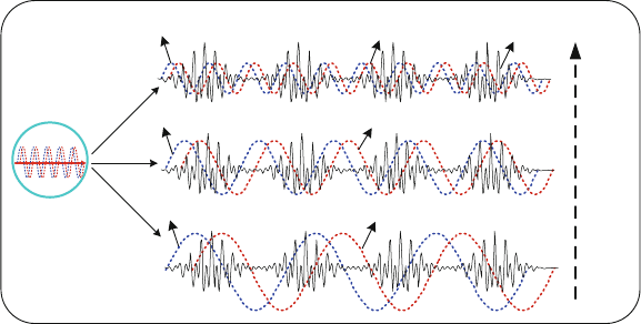
Equations (2.4) and (2.6) indicate that the Fourier transform is essentially a

convolution between the time series xðtÞ or x

and a series of sine and cosine

functions that can be viewed as template functions. The operation measures the

similarity betwee n xðtÞ or x

and the template functions, and expresses the average

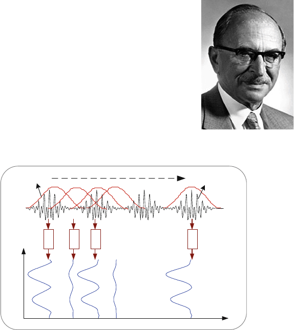
frequency information during the entire p eriod of the signal analyzed. In Fig. 2.3,

such an operation is graphically illustrated.

“An arbitrary function,

continuous or with

discontinuities, defined in a finite

interval by an arbitrarily

capricious graph can always be

expressed as a sum of sinusoids”

J.B.J. Fourier

Fig. 2.2 Jean B. Joseph Fourier (1768 1830)

2.1 Fourier Transform 19

To compute the DFT of a signal with N samples, multiplication of an N  N

matrix that contains the primitive nth root of unity e

i2p=N

by the signal is needed.

Such an operation takes a total of arithmetic operations on the order of N

complete. The computational time increases quickly as the number of the samples

increases. For exampl e, a time series of N ¼ 256 (i.e., 2

) samples takes 65,536

operational steps to complete, whereas for N ¼ 4,096 (i.e., 2

), a total of

16,777,216 steps will be needed to compute its DFT. The high computational

cost limited the widespread application of the DFT in its early stage, until a more

efﬁcient algorithm, called the Cooley Tukey algorithm, was introduced in 1965

(Cooley and Tukey 1965). This algorithm is also called the fast Fourier transform

(FFT), and what it does is to recursively break down a DFT of a large data sample

(i.e., a large N) into a series of smaller DFTs of smaller samples by dividing the

transform with size N into two pieces of size N/2 at each step, and reduce the

arithmetic operations to a total of N logðNÞ. Comparing to the N

operations

required for DFT, this represents a time reduction of up to 96%, when, for example,

the data sample number N is 256.

In practice, the phenomena of leakage and aliasing can happen during the

calculation of DFT (Ko

rner 1988). Leakage is caused by the discon tinuities

involved when a signal is extended periodically for performing the DFT. Applying

a window to the signal to force it to contain a full period can prevent leakage from

happening. However, the window itself may contribute frequency information to

the signal. Aliasing occurs when the Shannon’s sampling theorem is violated,

(Bracewell 1999) causing the actual frequency component to appear at different

locations in the frequenc y spectrum. This can be solved by ensuring the sampling

frequency to be at least twice as large as the maximum frequency component

contained in the signal (Bracewell 1999). This requires, however, that the maxi-

mum frequency component is known a priori.

The Fourier transform of the signal shown in Fig. 2.1 is illustrated in Fig. 2.4.

The ﬁgure shows two major fre quency peaks at 650 and 1,500 Hz, respectively.

j2π

cos(2p f

sin(2p f

cos(2p f

•

x(t)

Fig. 2.3 Illustration of the Fourier transform of a continuous signal x(t)

20 2 From Fourier Transform to Wavelet Transform: A Historical Perspective

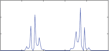
However, it does not reveal how the signal’s frequenc y contents vary with time;

that is, the ﬁgure does not reveal if the two frequency components are continuously

present throughout the time of observation or only at certain intervals, as is

implicitly shown in the time-domain representation. Because the temporal structure

of the signal is not reve aled, the merit of the Fourier transform is limited; speciﬁ-

cally, it is not suited for analyzing nonstationary sign als. On the other hand, as

signals encountered in manufacturing are generally nonstationary in nature (e.g.,

subtle, time-localized changes caused by structural defects are typically seen in

vibration signals measured from rotary machines), a new signal processing tech-

nique that is able to handle the nonstationarity of a signal is needed.

2.2 Short-Time Fourier Transform

A straightforward solution to overcoming the limitations of the Fourier transform is

to introduce an analysis window of certain length that glides through the signal

along the time axis to perform a “time-localized” Fourier transform. Such a concept

led to the short-time Fourier transform (STFT), introduced by Dennis Gabor

(Fig. 2.5) in his paper titled “Theory of communication,” published in 1946

(Gabor 1946).

As shown in Fig. 2.6, the STFT emp loys a slidi ng window function g(t)

that is centered at time t. For each speciﬁc t, a time-localized Fourier transform

is performed on the signal x(t) within the window. Subsequently, the window

is moved by t along the time line, and another Fourier transform is performed.

Through such consecutive operations, Fourier transform of the entire signal can

be performed. The signal segment within the window function is assumed to

be approximately stationary. As a result, the STFT decomposes a time domain

signal into a 2D time-frequency representation, and variations of the frequenc y

content of that signal within the window function are revealed, as illustrated in

Fig. 2.6.

0 400 800 1200 1600 2000

100

150

Frequency (Hz)

Magnitude

=650 Hz

=1500 Hz

Fig. 2.4 Fourier transform results of the signal x(t)

2.2 Short Time Fourier Transform 21

Using the inner product notation as before, the STFT can be expressed as

STFTð t ; f Þ¼hx; g

t; f

i¼

xðtÞg



t; f

ðtÞdt ¼

xðtÞgðt  tÞe

j2pft

dt (2.8)

Equation (2.8) can also be viewed as a measure of “similarity” between the signal

xðtÞ and the time-shifted and frequency-modulated window function gðtÞ. Over the

past few decades, various types of window functions have been developed (Oppen-

heim et al. 1999), and each of them is speciﬁcally tailored toward a particular type

of appl ication. For example, the Gaussian window designed for analyzing transient

signals, and the Hamming and Hann windows are appl icable to narrowband,

random signals, and the Kaiser-Bessel window is better suited for separating two

signal components with frequencies very close to each other but with widely

differing amplitudes. It should be noted that the choice of the window function

Time Shift

g(t)

Time

Frequency

FFT

•

x(t)

Fig. 2.6 Illustration of short time Fourier transform on the test signal x( t)

Fig. 2.5 Dennis Gabor

(1900 1979)

22 2 From Fourier Transform to Wavelet Transform: A Historical Perspective

directly affects the time and frequency resolutions of the analysis result. While

higher resolution in general provides better separation of the constituent compo-

nents within a signal, the time and frequency resolutions of the STFT technique

cannot be chosen arbitrarily at the same time, according to the uncertainty principle

(Cohen 1989). Speciﬁcally, the product of the time and frequency resolutions is

lower bounded by

Dt  Df 

(2.9)

where Dt and Df denote the time and frequency resolutions, respectively. Analyti-

cally, the time resolution Dt is measured by the root-mean-square time width of the

window function, deﬁned as

jgðtÞj

(2.10)

Similarly, the frequency resolution Df is measured by the root-mean-square band-

width of the window function, and is deﬁned as (Rioul and Vetterli 1991)

jGðf Þj

(2.11)

In (2.11), Gð f Þ is the Fourier transform of the window function g(t). As

an example, the Gaussian window function gðtÞ¼e

(with a being a constant

and t controlling the window width) has the time and frequency resolutions of

Dt ¼ t=ð2 a

Þ and Df ¼ a

=ðt  2 pÞ, respectively. As a result, the time-frequency

resolution provided by the Gaussian window when analyzing a signal x(t)

is Dt  Df ¼ 1=4p. As the time and frequency resolutions of a window function

are dependent on the parameter t only, once the window function is chosen,

the time and frequency resolutions over the entire time-frequency plane are

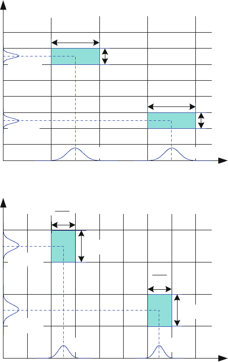
ﬁxed. Illustrated in Fig. 2.7 are two scenarios where the products of the time and

frequency resolutions of the window function (i.e., the area deﬁned by the

product of Dt  Df ) are the same, regardless of the actual window size (t or t=2)

employed.

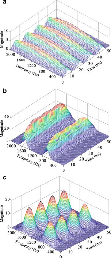
The effect of the window size t on the time and frequency resolution s is

illustrated in Fig. 2.8, where STFT with the Gaussian window was performed

on the signal show n in Fig. 2.1. Altogether three different window sizes (i.e., 1.6,

6.4, and 25.6 ms) were chosen. While the smallest window width of 1.6 ms

has provided high time resolution in separating the four pulse trains contained

in the signal, as illustrated in Fig. 2.8 a, its frequency resolution was too low

to differentiate the two time-overlapped transient elements within each group.

As a result, the frequency ele ments 1,500 and 650 Hz are displayed as one

lumped group on the time-frequency plane. In contrast, the largest window width

2.2 Short Time Fourier Transform 23

of 25.6 ms provided good frequency resolutio n to illustrate the two frequency

components in Fig. 2.8b. However, the time-resolution was insufﬁcient to differen-

tiate the four pulse trains that are timely separated with a 12-ms interval. The

best overall performance is given by the window width of 6.4 ms, shown in

Fig. 2.8c, which allowed for all of the transients to be adequately differentiated

on the time -frequency plane. Given that the speciﬁc frequency content of an

Δf

2Δf

2Δ

Δt

, f

( f )|

, f

( f )|

, f

( f )|

, f

( f )|

, f

(t)|

, f

(t)|

, f

(t)|

, f

(t)|

Window size: t

Window size: t /2

3 t

Fig. 2.7 Time frequency resolutions associated with the STFT technique. (a) Window size t and

(b) window size t/2

24 2 From Fourier Transform to Wavelet Transform: A Historical Perspective

experimentally measured signal is generally not known a priori, selection of

a suitable window size for effective signal decomposition using the STFT technique

is not guaranteed. The inherent drawback of the STFT motivates researchers

to look for other techniques that are better suited for proce ssing nonstationary

signals. One of such techniques, which is the focus of this book, is the wavelet

transform.

Fig. 2.8 Results of the STFT

of the signal using three

different window sizes.

(a) Window size 1.6 ms,

(b) window size 25.6 ms, and

2.2 Short Time Fourier Transform 25

2.3 Wavelet Transform

From a historical point of view, the ﬁrst reference to the wavelet goes back to

the early twentieth century when Alfred Haar (Fig. 2.9) wrote his dissertation titled

“On the theory of the orthogonal function systems” in 1909 to obtain his doctoral

degree at the University of Go

ttingen. His research on orthogonal systems of

functions led to the development of a set of rectangular basis functions (Haar

1910), as illustrated in Fig. 2.10. Later, an entire wavelet family, the Haar wavelet,

was named on the basi s of this set of functions, and it is also the simplest wavelet

family developed till this date.

Essentially, Haar’s basis function consists of a short positive pu lse followed by

a short negative pulse, and it was used to illustrate a countable orthonormal system

for the space of square-integrable functions on the real line (Haar 1910). Later, the

Haar basis function was applied to compress images (DeVore et al. 1992).

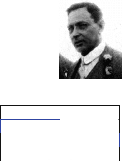
Little advancement in the ﬁeld of wavelets was reported after Haar’s work, until

a physicist, Paul Levy (Fig. 2.11), investigated the Brownian motion in the 1930s.

He discovered that the scale-varying function, that is, the Haar basis function,

was better suited than the Fourier basis functions for studying subtle details in

the Brownian motion. In addition, the Haar basis function can be scaled into

different intervals, such as the interval [0, 1] or the intervals [0, 1/2] and [1/2, 1],

thereby providing higher precision when modeling a function than that provided by

the Fourier basis function, as it can only have one interval [ 1, 1].

Fig. 2.9 Alfred Haar

(1885 1933)

0 0.2 0.4 0.6 0.8 1

-2

-1

Time (ms)

Amplitude

Fig. 2.10 The rectangular

basis function

26 2 From Fourier Transform to Wavelet Transform: A Historical Perspective

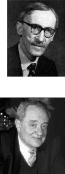
While several individual s, such as John Littlewood, Richard Paley (Littlewood

and Paley 1931), Elias M. Stein (Jaffard et al. 2001), and Norman H. Ricker

(Ricker 1953) have contributed, from the 1930s to the 1970s, to advancing

the state of research in wavelets as it is called today, major advancement in the

ﬁeld was attributed to Jean Morlet (Fig. 2.12) who developed and implemented

the technique of scaling and shifting of the anal ysis window functions in analyz-

ing acoustic echoes while working for an oil company in the mid 1970s (Mackenzie

2001). By sending acoustic impulses into the ground and analy zing the

received echoes, the existence of oil beneath the earth crust as well as the thickness

of the oil layer can be identiﬁed. When Morlet ﬁrst used the STFT to analyze

these echoes, he found that keepi ng the width of the window function ﬁxed

did not work. As a solution to the problem, he experimented with keeping

the frequency of the window function constant while changing the width of the

window by stretching or squeezing the window function (Mackenzie 2001). The

resulting waveforms of varying widths were called by Morlet the “Wavele t”, and

this marked the beginning of the era of wavelet research. As a matter of fact,

the approach that Morlet used was similar to what Haar did before, but the

theoretical formation of the wavelet transform was ﬁrst proposed only after

Jean Morlet teamed up with Alex Grossmann to work out the idea that a signal

could be transformed into the form of a wavelet and then transformed back into its

original form without any information loss (Grossmann and Morlet 1984).

Fig. 2.11 Paul Levy

(1886 1971)

Fig. 2.12 Jean Morlet

(1931 2007)

2.3 Wavelet Transform 27