Gerya T. Introduction to Numerical Geodynamic Modelling
Подождите немного. Документ загружается.

17.10 Mantle convection with phase changes 297
fields of geodynamic modelling in terms of both technical and conceptual pro-
gresses (e.g., Yuen et al., 2000). Realistic modelling of terrestrial and planetary
convection is a challenging topic (e.g., Hansen and Yuen, 1988; Larsen et al.,
1995; Yuen et al., 2000; Zhong et al., 2007; Tackley, 2008) and requires the appli-
cation of sophisticated 3D numerical codes working with spherical geometries at
high grid resolution which can almost exclusively only be preformed by parallel
computing on ‘big machines’. Indeed, one important aspect of modelling mantle
convection, which is of interest for this chapter, is the incorporation of solid-state
phase transitions into such numerical models.
Solid-state phase transitions are crucial phenomena in the Earth’s mantle. Major
phase transitions include olivine–spinel at 410 km depth and spinel–perovskite
at 670 km depth. These transitions are associated with significant changes in
mantle density and seismic wave speeds (Turcotte and Schubert, 2002). It was
also suggested recently, that the so-called D
(D-double-prime) discontinuity near
the core–mantle boundary is related to perovskite–post-perovskite phase transition
(Oganov and Ono, 2004; Murakami et al., 2004). Phase transitions affect the
dynamics of mantle convection due to (1) density changes and (2) latent heating
(Richter, 1973; Schubert et al., 1975; Christensen and Yuen, 1985; Tackley, 1993;
Zhong and Gurnis, 1994).
Phase changes are traditionally included in mantle convection models (e.g.,
Richter, 1973; Schubert et al., 1975; Christensen and Yuen, 1985; Tackley, 1993;
Zhong and Gurnis, 1994) by programming each transition individually (i.e. sim-
ilarly to what we did with melting reactions in the previous example). However,
for realistic mantle compositions, the amount of various phase transitions is larger
than only three (Fig. 17.10) and these phase transitions involve several minerals
of variable composition (so called solid solutions, Table 17.3) which makes the
traditional approach quite inconvenient. An alternative method has been developed
recently based on Gibbs free energy minimisation (Chapter 2). This method was
initially applied for crustal- and lithospheric-scale thermal (Petrini et al., 2001;
Gerya et al., 2001; Kaus et al., 2005) and thermomechanical (Gerya et al., 2004c,
2006; Yamato et al., 2008) models and then expanded to mantle convection models
(Tackley, 2008).
The idea of this petrological-thermomechanical method is relatively simple
(Gerya et al., 2004c; 2006): (i) phase diagrams (P–T pseudosections) and related
density (ρ) and enthalpy (H) maps (see programming exercise 2.3; Chapter 2) are
first computed for the necessary rock compositions in a relevant range of P–T
conditions and (ii) these maps are then used in thermomechanical experiments for
computing density (ρ), effective heat capacity incorporating latent heat (C
Peff
)and
energetic effects (both adiabatic and latent heating) for isothermal (de)compression
(H
P
) for material points (markers) based on standard thermodynamic formulas and
298 Design of 2D numerical geodynamic models
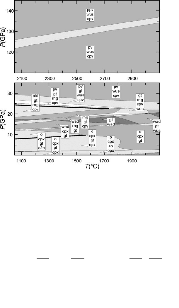
Fig. 17.10 Phase relations for the CaO-FeO-MgO-Al
2
O
3
-SiO
2
pyrolite model
(see Table 17.3 for notations of minerals) computed (Mishin et al., 2008) with the
Gibbs free energy minimisation program Perple_X (Connolly, 2005). To permit
the resolution of phase relations the diagram is split to exclude the large depth
interval between the transition zone and core–mantle boundary in which the model
does not predict phase transformations. Composition for the pyrolite model is
3.87 wt% CaO, 8.11 wt% FeO, 3.61 wt% Al
2
O
3
, 38.59 wt% MgO and 45.82 wt%
SiO2.
numerical differentiation in P–T space (Fig. 17.11)
ρ = ρ
i,j
1 −
T
m
T
1 −
P
m
P
+ ρ
i+1,j
1 −
T
m
T
P
m
P
+ρ
i,j+1
T
m
T
1 −
P
m
P
+ ρ
i+1,j +1
T
m
T
P
m
P
, (17.20)
Cp
eff
=
∂H
∂T
P =const
=
H
i,j+1
− H
i,j
T
1 −
P
m
P
+
H
i+1,j +1
− H
i+1,j
T
P
m
P
,
(17.21)
17.10 Mantle convection with phase changes 299
Table 17.3 Phase notation and formulae of minerals for the
CaO-FeO-MgO-Al
2
O
3
-SiO
2
pyrolite model (Fig. 17.9)
Symbol Phase Formula
∗
aki akimotoite Mg
x
Fe
1–x–y
Al
2y
Si
1–y
O
3
, x + y ≤ 1
c2c pyroxene [Mg
x
Fe
1–x
]
4
Si
4
O
12
cpv Ca–perovskite CaSiO
3
cpx clinopyroxene Ca
2y
Mg
4–2x–2y
Fe
2x
Si
4
O
12
gt garnet Fe
3x
Ca
3y
Mg
3(1–x+y+z/3)
Al
2–2z
Si
3+z
O
12
, x + y ≤ 1
o olivine [Mg
x
Fe
1–x
]
2
SiO
4
opx orthopyroxene [Mg
x
Fe
1–x
]
4–2y
Al
4(1–y)
Si
4
O
12
ppv post–perovskite Mg
x
Fe
1–x–y
Al
2y
Si
1–y
O
3
, x + y ≤ 1
pv perovskite Mg
x
Fe
1–x–y
Al
2y
Si
1–y
O
3
, x + y ≤ 1
rng ringwoodite [Mg
x
Fe
1–x
]
2
SiO
4
sp spinel Mg
x
Fe
1–x
Al
2
O
3
wad waddsleyite [Mg
x
Fe
1–x
]
2
SiO
4
wus magnesiowuestite Mg
x
Fe
1–x
O
∗
Unless otherwise noted, the compositional variables w, x, y, and z may
vary between zero and unity and are determined as a function of pressure
and temperature by free-energy minimisation with Perple
X program (Connolly,
2005).
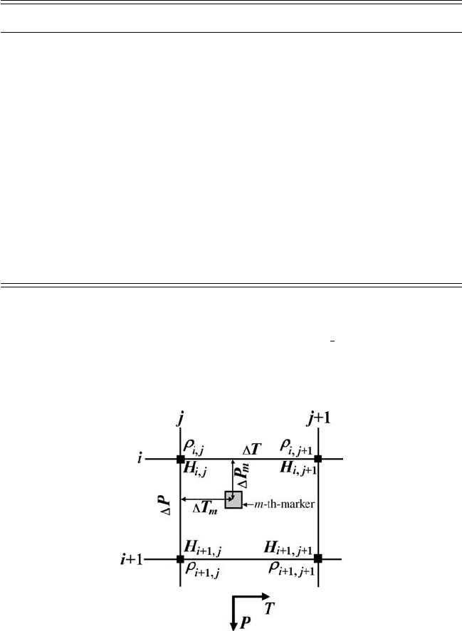
Fig. 17.11 Stencil associated with the P–T grid used for the interpolation
of physical properties from enthalpy and density look-up tables, to the
markers.

300 Design of 2D numerical geodynamic models
H
P
DP/Dt
=
1 − ρ
∂H
∂P
T =const
= 1 −
H
i+1,j
− H
i,j
P
1 −
T
m
T
ρ
i+1,j
+ ρ
i,j
2
−
H
i+1,j +1
− H
i,j+1
P
T
m
T
ρ
i+1,j +1
+ ρ
i,j+1
2
. (17.22)
The temperature equation (9.8) is respectively modified as
ρC
Peff
DT
Dt
=−
∂q
i
∂x
i
+ H
r
+ H
s
+ H
P
. (17.23)
The stable mineralogy and physical properties for the mantle used in our example
are computed (Mishin et al., 2008) with Perple_X (Connolly, 2005) by a free
energy minimisation approach. For this purpose the Mie-Grueneisen formulation
of Stixrude and Bukowinski (1990) was adopted with the parameterisation of
Stixrude and Lithgow-Bertelloni (2005) augmented for lower mantle phases as
described by Khan et al. (2006). This parameterisation limits the chemical model
to the CaO-FeO-MgO-Al
2
O
3
-SiO
2
(Table 17.3). The mantle rheology is based
on the dry olivine flow law (Table 17.1) with an activation volume of 5 cm
3
,
which allows us to mimic 1.5–3 order of magnitude increase in viscosity for the
lower mantle. This range is often used in mantle convection models (e.g. Tackley,
2000). Olivine is obviously not stable in the deep mantle below the olivine–spinel
transition and, therefore, our rheological choice is rather arbitrary. This is related
to the limited availability of experimentally calibrated flow laws applicable to the
deep mantle such that simplified temperature- and depth-dependent rheological
models are traditionally used in numerical mantle convection studies (e.g., Richter,
1973; Schubert et al., 1975; Christensen and Yuen, 1985; Zhong and Gurnis, 1994;
Tackley, 1993, 2000, 2008).
Figure 17.12 shows several stages of a mantle convection modelled with the code
Mantle_convection.m. The model design is simple: a square 3000 ×3000 km box
with free slip boundaries, constant temperature conditions applied at the top and
in the bottom and no heat flux condition across the vertical walls. In this model
we do not intend to model self-consistent plate generation (e.g. Tackley, 2000)
and therefore use uniform, relatively coarse grid resolution. Mantle convection is
characterised by a semi-layered structure with a strongly convecting upper part
(above 670 km depth) and a much more slowly deforming lower mantle with
several plumes penetrating from the core–mantle boundary (Figs. 17.12, 17.13(b)).
Density changes (Fig. 17.13(d)) and thermal effects (Fig. 17.13(c)) of various
phase transitions (Fig. 17.10) are captured with our petrological-thermomechanical
numerical approach without programming them individually. This approach makes
coding simpler and easily allows changes to be made in the case of testing different
models for mantle composition.
17.11 Deformation of self-gravitating planetary body 301
(a) (b) (c)
(d) (e) (f)
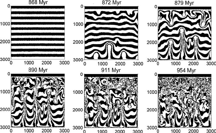
Fig. 17.12 Development of mantle convection processes with phase changes
(Fig. 17.10) computed with the petrological-thermomecanical code Mantle_
convection.m associated with this chapter. Model resolution is 51 ×51 nodal
points with 40 000 randomly distributed markers. Grid resolution is uniform in
both directions. The model is shown from an arbitrary stage of 868 Myr when
non-compositional layering is superimposed for visualising deformation onto a
pre-computed non-steady thermal structure. Note, moderate deformation of the
lower mantle by localised upwellings and downwellings (thermal plumes) which
contrasts with the intense chaotic mixing of the upper mantle.
17.11 Deformation of self-gravitating planetary body
Lastly, let us discuss some planetary-scale applications of numerical geodynamic
modelling which are becoming more and more widespread in relation to the
problem of planetary accretion and core formation processes (e.g. Stevenson,
1981). One important group of such applications concerns the internal deformation
of an inhomogeneous, self-gravitating body. Numerical modelling of deformation
of such a body was already discussed in Chapter 11 with the use of a ‘spherical-
Cartesian’ approach (Honda et al., 1993; Gerya and Yuen, 2007; Lin et al., 2009).
This approach is relatively simple and does not require major rewriting of the
Cartesian code used for the previous examples. All that is required is to add the
numerical solution of the Poisson equation before solving the momentum and
continuity equations (Fig. 11.3). Gravitational acceleration components are then
computed from the gravity potential locally and are used in the right-hand side
of the momentum equation (Eqs. (11.18), (11.19)). As a boundary condition for
gravity potential, one can use constant gravitational potential value (e.g. = 0)
302 Design of 2D numerical geodynamic models
(a) (c)
(d)(b)
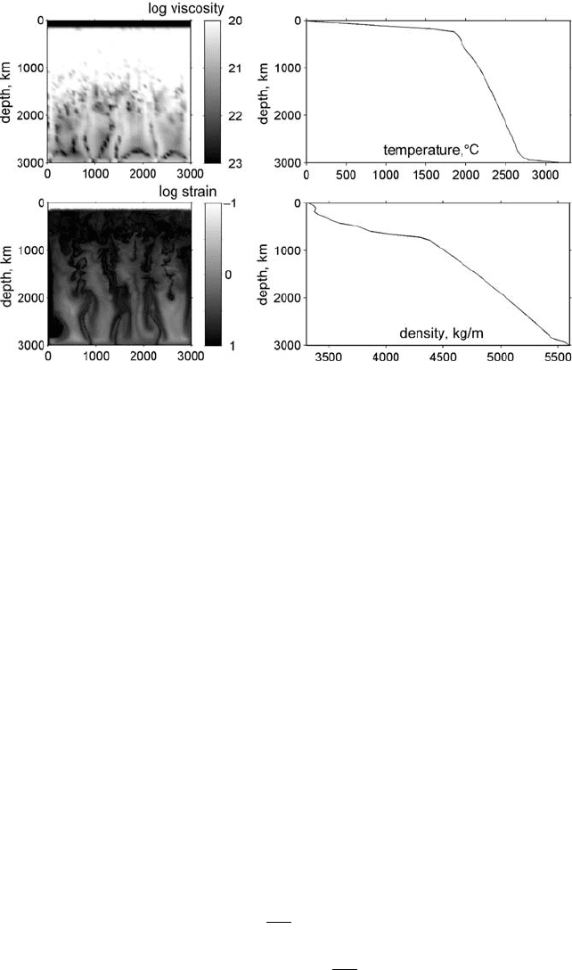
Fig. 17.13 Viscosity (a) and strain (b) maps and horizontally averaged temperature
(c) and density (d) profiles for the computed mantle convection model at 954 Myr
(Fig. 17.12(f)). Note, 1–2 order of magnitude viscosity contrast between the upper
and lower mantle obtained with our simplified rheological model based on dry
olivine flow law with activation volume of 5 cm
3
. Mantle deformation in (b) is
semi-layered and is strongly affected by the spinel–perovskite transition at around
670 km depth due to its negative Clapeyron slope (Fig. 17.10) which creates
difficulties for both upwellings and downwellings for penetrating this boundary.
Cold lithosphere at the top of the model remains undeformed (stagnant lid regime,
e.g. Tackley, 2000) due to the prescribed high plastic strength (sin(ϕ) =0.6) which
corresponds to a dry mantle. Plate bending processes (Fig. 17.1) in this lithosphere
are not modelled due to the imposed free slip upper boundary condition without a
weak layer (in contrast to free-surface condition formed by sticky air/water used in
all previous examples) as well as due to the very coarse grid resolution employed
here (60 × 60 km in contrast to 2 × 2 km needed for properly resolving slab
bending processes).
applied at a circular surface located at a distance from the planet (Fig. 14.7,
Eq. (14.12)). The chosen value of the potential along the surface is arbitrary since
it does not affect the resulting gravitational acceleration field (given by derivatives
of the potential). The use of such a boundary condition is based on the fact that with
growing distance from the planet, both the gravitational acceleration and gravity
potential tend to become solely a function of the planetary mass (m
p
)andthe
distance to its centre (d)
g = G
m
p
d
2
, (17.24)
= const − G
m
p
d
. (17.25)
17.11 Deformation of self-gravitating planetary body 303
However, it should be mentioned that forcing the potential to be uniform outside
the planet at a certain distance from the planetary centre also affects the gravitational
field inside the planet (especially its tangential component). Therefore, the gravity
potential boundary should preferably be located at a significant distance from the
planetary surface which should be comparable to the planetary radius (Lin et al.,
2009).
The initial setup for the numerical experiment on gravitational redistribution
of metal and silicate in a Mars-sized body (3000 km in radius) is shown in
Figure 17.14 (0.03 Myr). This setup is based on the numerical study of Golabek
et al. (2008a) who investigated rheological controls on the terrestrial core forma-
tion mechanism. The initial temperature is 273 K at the surface and 1200 K at
100 km depth and then rises linearly to 1500 K in the centre of the planet. This
initial profile is rather arbitrary and mimics to some degree the effects of various
planetary heating processes: (i) decay of short-lived radioactive isotopes (MacPher-
son et al., 1995) such as
26
Al (half-life time is 0.73 Ma) and
60
Fe (half-life time is
1.5 Ma), (ii) impact heating by accreted planetesimals (Davies, 1985; Melosh,
1990), (iii) impact associated gravitational unloading (Asphaug et al., 2006) and
(iv) adiabatic heating caused by growing pressure in the planetary interior. The
planet is heterogeneous and composed of a silicate matrix and randomly dis-
tributed iron diapirs with radii varying from 50 to 100 km. Using a variable-sized
diapir is related to the fact that the size distribution of the planetesimals and plane-
tary embryos after runaway growth and the formation of Mars-sized bodies should
be heterogeneous (Melosh, 1990; Tonks and Melosh, 1992; Stevenson, 2008). As
in the previous example, we also apply a coupled petrological-thermomechanical
approach for modelling density and thermal properties of the silicate matrix, which
is assumed to have pyrolitic composition (Fig. 17.10). The rheology of silicate
corresponds to dry olivine (Table 17.1) with an activation volume of 10 cm
3
. Con-
stant density (10000 kg/m
3
) and lowered viscosity (10
20
Pa s) are used for the
metal.
Viscosity of the weak mass less-like medium (1 kg/m
3
) surrounding the planet
is also taken to be 10
20
Pa s, which is 2–5 order of magnitude lower than that
of silicate at the planetary surface. This is sufficient to provide free surface like
condition (Schmeling et al., 2008; Lin et al., 2009). Lower viscosity will require
shorter time steps which is inconvenient. Feedback from shear heating caused
by gravitational energy release is also taken into account since this process may
strongly affect temperature distribution inside the differentiating planet (Gerya and
Yuen, 2007; Golabek et al., 2008a).
Figure 17.14 shows several stages of the core formation computed with the code
Core_formation.m associated with this chapter. Model development corresponds
to so called ‘decomposition mode’ (Golabek et al., 2008a) which is defined by
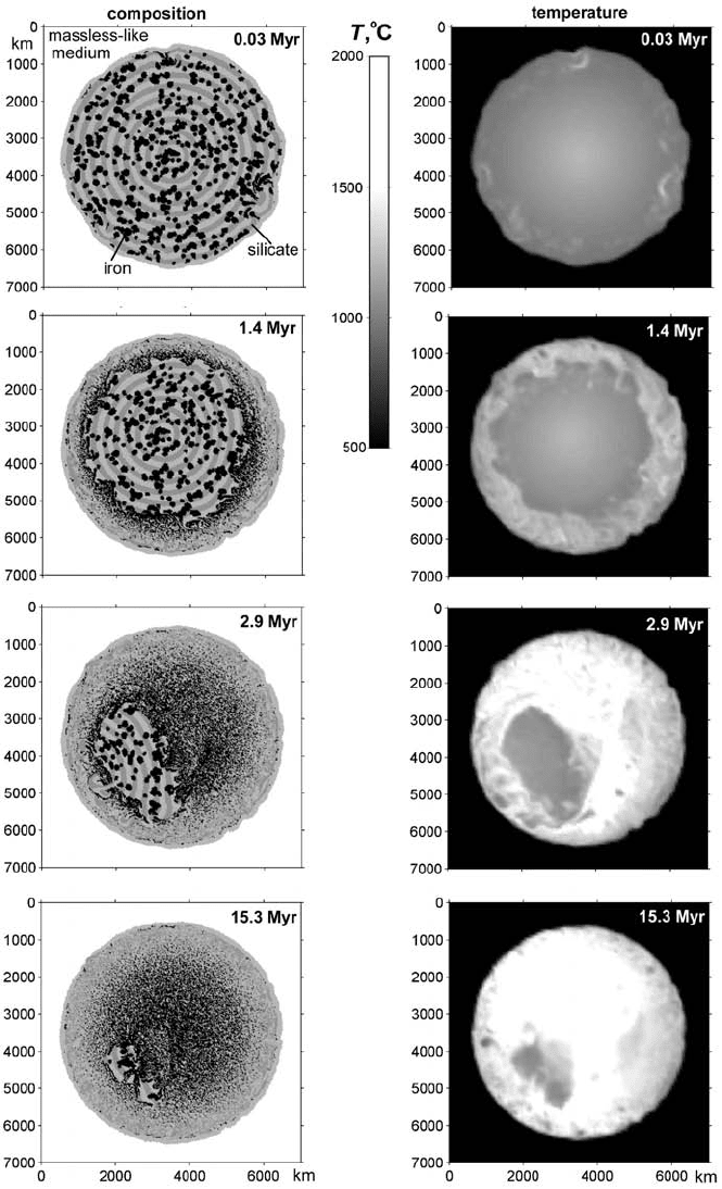
Fig. 17.14 Development of the compositional (left column) and temperature (right
column) fields in the numerical experiment on core formation computed with
the code Core_formation.m associated with this chapter. Model resolution is
101 ×101 nodal points with 160 000 randomly distributed markers.
17.11 Deformation of self-gravitating planetary body 305
choosing a relatively large activation volume (10 cm
3
) and plastic strength (no
Peierls plasticity limit is imposed) of the silicate matrix that effectively makes the
pressurised planetary interior rheologically stronger than the outer shell. Therefore,
in this model, the iron diapirs near the surface are activated foremost (Fig. 17.14,
0.03 Myr). Even the slightest asymmetries in the initial iron distribution lead to
an earlier initiation of diapir sinking in some distinct regions where significantly
larger temperatures develop due to shear heating processes. The diapir sinking
releases large amounts of energy. This leads to the activation of neighbouring
diapirs and finally to the formation of large iron ponds. The underlying material
of the planetary interior is too strong to be deformed by stresses arising from the
available iron agglomerations. Therefore, all iron diapirs in the outer region of
the planet will be finally activated. This leads to a global temperature rise in the
upper layers of the planet (Fig. 17.14, 1.4 Myr). Consequently, a low-viscosity
shell, basically analogous to a magma ocean, is formed around the remaining
highly viscous central region. The iron ponds on top of this high-viscosity sphere
finally coalescence and form an iron-rich ring around the central region (Fig.
17.14, 1.4 Myr), as was suggested by Stevenson (1981) and Ida et al. (1987).
Temperature and density dis-equilibrium around the ring leads to the degree-one
instability (e.g. Ida et al., 1987) resulting in the formation of advective streams
of the iron-rich material around the central region. Asymmetry of these flows
causes and sustains the rotation of the central sphere and the resulting shear heat-
ing aids in further decomposition (Fig. 17.14, 2.9 Myr). Iron accumulating on
the one side of the planet pushes the stiff, non-differentiated planetary interior
(including the passive iron diapirs) out of the central region creating a noticeable
asymmetry in the planet (Fig. 17.14, 2.9 Myr). A similar scenario was proposed
by Elsasser (1963) and modelled numerically in a simplified way (Honda et al.,
1993; Lin et al., 2009), but under the assumption of a cold central region. This
translation favours the decompression-related decomposition of the ‘exhuming’
interiors when the material approaches shallower depths. Decompression causes
(via activation volume) a viscosity reduction in the regions of the translated cen-
tral sphere closer to the planet’s surface. The silicates released at the leading
side, rise due to their low density as Rayleigh–Taylor instabilities upwards into
the high-temperature zone (Fig. 17.14, 2.9 Myr). This causes further iron release
and makes the process of interior ‘decomposition’ self-sustaining, which finally
results in the formation of an iron core (Fig. 17.14, 15.3 Myr). Obviously, this
scenario is non-unique and several others core formation modes may develop
instead, depending on variations in planetary size, temperature structure and
material properties, and particularly the effective silicate rheology (Golabek et al.,
2008a).
306 Design of 2D numerical geodynamic models
Programming exercise and homework
Exercise 17.1
Program a model for extension of a continental lithosphere based on the provided
oceanic lithosphere extension model (Fig. 17.4). Take the initial compositional and
thermal structure of the continental lithosphere to be the same as in the continental
collision example (Fig. 17.5(a)). Use the codes Extension.m and Collision.m
associated with this chapter. Alternatively, you may also want to program a similar
model using a uniform grid resolution by using your own visco-elasto-plastic codes
created during exercises for Chapter 13.