Greene W.H. Econometric Analysis

Подождите немного. Документ загружается.

CHAPTER 12

✦

Estimation Frameworks in Econometrics

439

More intricate speciﬁcations use the negative binomial model (version 2, NB2),

Prob[Y = y |x] =

( y + α)

( α)( y + 1)



λ + α





λ + α



, y = 0, 1, ...,

where α is an overdispersion parameter. (See Section 18.4.) A satisfactory, appropriate speci-

ﬁcation for bivariate outcomes has been an ongoing topic of research. Early suggestions were

based on a latent mixture model,

= z + w

where w

and w

have the Poisson or NB2 distributions speciﬁed earlier with conditional

means λ

and λ

and z is taken to be an unobserved Poisson or NB variable. This formulation

induces correlation between the variables but is unsatisfactory because that correlation must

be positive. In a natural application, y

is doctor visits and y

is hospital visits. These could

be negatively correlated. Munkin and Trivedi (1999) speciﬁed the jointness in the conditional

mean functions, in the form of latent, common heterogeneity;

= exp(x



+ ε)

where ε is common to the two functions. Cameron et al. (2004) used a bivariate copula

approach to analyze Australian data on self-reported and actual physician visits (the lat-

ter maintained by the Health Insurance Commission). They made two adjustments to the

preceding model we developed above. First, they adapted the basic copula formulation to

these discrete random variables. Second, the variable of interest to them was not the actual

or self-reported count, but the difference. Both of these are straightforward modiﬁcations of

the basic copula model.

12.3 SEMIPARAMETRIC ESTIMATION

Semiparametric estimation is based on fewer assumptions than parametric estimation.

In general, the distributional assumption is removed, and an estimator is devised from

certain more general characteristics of the population. Intuition suggests two (correct)

conclusions. First, the semiparametric estimator will be more robust than the parametric

estimator—it will retain its properties, notably consistency across a greater range of

speciﬁcations. Consider our most familiar example. The least squares slope estimator is

consistent whenever the data are well behaved and the disturbances and the regressors

are uncorrelated. This is even true for the frontier function in Example 12.2, which has

an asymmetric, nonnormal disturbance. But, second, this robustness comes at a cost.

The distributional assumption usually makes the preferred estimator more efﬁcient

than a robust one. The best robust estimator in its class will usually be inferior to the

parametric estimator when the assumption of the distribution is correct. Once again,

in the frontier function setting, least squares may be robust for the slopes, and it is

the most efﬁcient estimator that uses only the orthogonality of the disturbances and

the regressors, but it will be inferior to the maximum likelihood estimator when the

two-part normal distribution is the correct assumption.

12.3.1 GMM ESTIMATION IN ECONOMETRICS

Recent applications in economics include many that base estimation on the method

of moments. The generalized method of moments departs from a set of model based

440

PART III

✦

Estimation Methodology

moment equations, E [m(y

, x

, β)] = 0, where the set of equations speciﬁes a relation-

ship known to hold in the population. We used one of these in the preceding paragraph.

The least squares estimator can be motivated by noting that the essential assumption is

that E [x

− x



β)] = 0. The estimator is obtained by seeking a parameter estimator,

b, which mimics the population result; (1/n)

− x



b)] = 0. These are, of course,

the normal equations for least squares. Note that the estimator is speciﬁed without ben-

eﬁt of any distributional assumption. Method of moments estimation is the subject of

Chapter 13, so we will defer further analysis until then.

12.3.2 MAXIMUM EMPIRICAL LIKELIHOOD ESTIMATION

Empirical likelihood methods are suggested as a semiparametric alternative to maxi-

mum likelihood. As we shall see shortly, the estimator is closely related to the GMM

estimator. Let π

denote generically the probability that y

takes the realized value in

the sample. Intuition suggests (correctly) that with no further information, π

will equal

1/n.Theempirical likelihood function is

EL =

i=1

1/n

The maximum empirical likelihood estimator maximizes EL. Equivalently, we maximize

the log of the empirical likelihood,

ELL =



i=1

ln π

As a maximization problem, this program lacks sufﬁcient structure to admit a solution—

the solutions for π

are unbounded. If we impose the restrictions that π

are probabilities

that sum to one, we can use a Langragean formulation to solve the optimization problem,

ELL =





i=1

ln π



+ λ



1 −



i=1



This slightly restricts the problem since with 0 <π

< 1 and 

= 1, the solution

suggested earlier becomes obvious. (There is nothing in the problem that differentiates

the π

’s, so they must all be equal to each other.) Inserting this result in the derivative

with respect to any speciﬁc π

produces the remaining result, λ = 1.

The maximization problem becomes meaningful when we impose a structure on the

data. To develop an example, we’ll recall Example 7.6, a nonlinear regression equation

for Income for the German Socioeconomic Panel data, where we speciﬁed

E[Income|Ag e , Sex, Educat ion] = exp(x



β) = h(x, β).

For purpose of an example, assume that Education may be endogenous in this equation,

but we have available a set of instruments, z, say (Age, Health, Sex, MarketCondition).

We have assumed that there are more instruments (4) than included variables (3), so that

the parameters will be overidentiﬁed (and the example will be complicated enough to

be interesting). (See Sections 8.3.4 and 8.6.) The orthogonality conditions for nonlinear

instrumental variable estimation are that the disturbances be uncorrelated with the

instrumental variables, so

E{z

[Income

− h(x

, β)]}=E[m

(β)] = 0.

CHAPTER 12

✦

Estimation Frameworks in Econometrics

441

The nonlinear least squares solution to this problem was developed in Section 8.6. A

GMM estimator will minimize with respect to β the criterion function

q =



(β)A

m(β)

where A is the chosen weighting matrix. Note that for our example, including the con-

stant term, there are four elements in β and ﬁve moment equations, so the parameters

are overidentiﬁed.

If we impose the restrictions implied by our moment equations on the empirical

likelihood function, instead, we obtain the population moment condition





i=1

(

Income

− h(x

, β)

)



= 0.

(The probabilities are population quantities, so this is the expected value.) This produces

the constrained empirical log likelihood

ELL =





i=1

ln π



+ λ



1 −



i=1



+ γ







i=1

(

Income

− h(x

, β)

)



The function is now maximized with respect to π

, λ, β (K elements) and γ (L ele-

ments, the number of instrumental variables). At the solution, the values of π

provide,

essentially, a set of weights. Cameron and Trivedi (2005, p. 205) provide a solution for

ˆπ

in terms of (β, γ ) and show, once again, that λ =1. The concentrated ELL function

with these inserted provides a function of γ and β that remains to be maximized.

The empirical likelihood estimator has the same asymptotic properties as the

GMM estimator. (This makes sense, given the resemblance of the estimation criteria—

ultimately, both are focused on the moment equations.) There is evidence that at least in

some cases, the ﬁnite sample properties of the empirical likelihood estimator might be

better than GMM. A survey appears in Imbens (2002). One suggested modiﬁcation of

the procedure is to replace the core function in (1/n)

ln π

with the entropy measure,

Entropy = (1/n)

ln π

The maximum entropy estimator is developed in Golan, Judge, and Miller (1996) and

Golan (2009).

12.3.3 LEAST ABSOLUTE DEVIATIONS ESTIMATION

AND QUANTILE REGRESSION

Least squares can be severely distorted by outlying observations in a small sample.

Recent applications in microeconomics and ﬁnancial economics involving thick-tailed

disturbance distributions, for example, are particularly likely to be affected by precisely

these sorts of observations. (Of course, in those applications in ﬁnance involving hun-

dreds of thousands of observations, which are becoming commonplace, this discussion

is moot.) These applications have led to the proposal of “robust” estimators that are

unaffected by outlying observations. One of these, the least absolute deviations, or LAD

estimator discussed in Section 7.3.1, is also useful in its own right as an estimator of the

conditional median function in the modiﬁed model

Med[y|x] = x



.50

442

PART III

✦

Estimation Methodology

That is, rather than providing a robust alternative to least squares as an estimator of

the slopes of E[y|x], LAD is an estimator of a different feature of the population. This

is essentially a semiparametric speciﬁcation in that it speciﬁes only a particular feature

of the distribution, its median, but not the distribution itself. It also speciﬁes that the

conditional median be a linear function of x.

The median, in turn, is only one possible quantile of interest. If the model is extended

to other quantiles of the conditional distribution, we obtain

Q[y|x, q] = x



such that Prob[y < x



|x] = q, 0 < q < 1.

This is essentially a nonparametric speciﬁcation. No assumption is made about the dis-

tribution of y|x or about its conditional variance. The fact that q can vary continuously

(strictly) between zero and one means that there is an inﬁnite number of possible “pa-

rameter vectors.” It seems reasonable to view the coefﬁcients, which we might write

β(q) less as ﬁxed “parameters,” as we do in the linear regression model, than loosely

as features of the distribution of y|x. For example, it is not likely to be meaningful

to view β(.49) to be discretely different from β(.50) or to compute precisely a partic-

ular difference such as β(.5) − β(.3). On the other hand, the qualitative difference,

or possibly the lack of a difference, between β(.3) and β(.5) may well be an inter-

esting characteristic of the population. The quantile regression model is examined in

Section 7.3.2.

12.3.4 KERNEL DENSITY METHODS

The kernel density estimator is an inherently nonparametric tool, so it ﬁts more ap-

propriately into the next section. But some models that use kernel methods are not

completely nonparametric. The partially linear model in Section 7.4 is a case in point.

Many models retain an index function formulation, that is, build the speciﬁcation around

a linear function, x



β, which makes them at least semiparametric, but nonetheless still

avoid distributional assumptions by using kernel methods. Lewbel’s (2000) estimator

for the binary choice model is another example.

Example 12.4 Semiparametric Estimator for Binary Choice Models

The core binary choice model analyzed in Section 17.3, the probit model, is a fully parametric

speciﬁcation. Under the assumptions of the model, maximum likelihood is the efﬁcient (and

appropriate) estimator. However, as documented in a voluminous literature, the estimator of

β is fragile with respect to failures of the distributional assumption. We will examine a few

semiparametric and nonparametric estimators in Section 17.4.7. To illustrate the nature of

the modeling process, we consider an estimator suggested by Lewbel (2000). The probit

model is based on the normal distribution, with Prob[ y

= 1 |x

] = Prob[x



β + ε

> 0] where

∼ N[0, 1]. The estimator of β under this speciﬁcation will be inconsistent if the distribution

is not normal or if ε

is heteroscedastic. Lewbel suggests the following: If (a) it can be as-

sumed that x

contains a “special” variable, v

, whose coefﬁcient has a known sign–a method

is developed for determining the sign and (b) the density of ε

is independent of this vari-

able, then a consistent estimator of β can be obtained by regression of [y

− s( v

)]/ f (v

)

on x

where s(v

) = 1ifv

> 0 and 0 otherwise and f (v

) is a kernel density estimator

of the density of v

. Lewbel’s estimator is robust to heteroscedasticity and distribution.

A method is also suggested for estimating the distribution of ε

. Note that Lewbel’s estimator

is semiparametric. His underlying model is a function of the parameters β, but the distribution

is unspeciﬁed.

CHAPTER 12

✦

Estimation Frameworks in Econometrics

443

12.3.5 COMPARING PARAMETRIC AND SEMIPARAMETRIC

ANALYSES

It is often of interest to compare the outcomes of parametric and semiparametric mod-

els. As we have noted earlier, the strong assumptions of the fully parametric model come

at a cost; the inferences from the model are only as robust as the underlying assump-

tions. Of course, the other side of that equation is that when the assumptions are met,

parametric models represent efﬁcient strategies for analyzing the data. The alternative,

semiparametric approaches relax assumptions such as normality and homoscedasticity.

It is important to note that the model extensions to which semiparametric estimators

are typically robust render the more heavily parameterized estimators inconsistent. The

comparison is not just one of efﬁciency. As a consequence, comparison of parameter

estimates can be misleading—the parametric and semiparametric estimators are often

estimating very different quantities.

Example 12.5 A Model of Vacation Expenditures

Melenberg and van Soest (1996) analyzed the 1981 vacation expenditures of a sample of

1,143 Dutch families. The important feature of the data that complicated the analysis was that

37 percent (423) of the families reported zero expenditures. A linear regression that ignores

this feature of the data would be heavily skewed toward underestimating the response of

expenditures to the covariates such as total family expenditures (budget), family size, age,

or education. (See Section 19.3.) The standard parametric approach to analyzing data of this

sort is the “Tobit,” or censored, regression model:

∗

= x



β + ε

, ε

∼ N[0, σ

= max(0, y

∗

(Maximum likelihood estimation of this model is examined in detail in Section 19.3.) The model

rests on two strong assumptions, normality and homoscedasticity. Both assumptions can be

relaxed in a more elaborate parametric framework, but the authors found that test statistics

persistently rejected one or both of the assumptions even with the extended speciﬁcations.

An alternative approach that is robust to both is Powell’s (1984, 1986a, b) censored least

absolute deviations estimator, which is a more technically demanding computation based

on the LAD estimator in Section 7.3.1. Not surprisingly, the parameter estimates produced

by the two approaches vary widely. The authors computed a variety of estimators of β.A

useful exercise that they did not undertake would be to compare the partial effects from the

different models. This is a benchmark on which the differences between the different esti-

mators can sometimes be reconciled. In the Tobit model, ∂ E[ y

] /∂x

= ( x



β /σ)β (see

Section 19.3). It is unclear how to compute the counterpart in the semiparametric model,

since the underlying speciﬁcation holds only that Med[ε

] = 0. (The authors report on

the Journal of Applied Econometrics data archive site that these data are proprietary. As

such, we were unable to extend the analysis to obtain estimates of partial effects.) This high-

lights a signiﬁcant difﬁculty with the semiparametric approach to estimation. In a nonlinear

model such as this one, it is often the partial effects that are of interest, not the coefﬁcients.

But, one of the byproducts of the more “robust” speciﬁcation is that the partial effects are

undeﬁned.

In a second stage of the analysis, the authors decomposed their expenditure equation into

a “participation” equation that modeled probabilities for the binary outcome “expenditure =

0or> 0” and a conditional expenditure equation for those with positive expenditure. [In

Section 18.4.8, we will label this a “hurdle” model. See Mullahy (1986).] For this step, the

authors once again used a parametric model based on the normal distribution (the probit

model—see Section 17.3) and a semiparametric model that is robust to distribution and

heteroscedasticity developed by Klein and Spady (1993). As before, the coefﬁcient estimates

444

PART III

✦

Estimation Methodology

1.0

0.0

0.1

0.2

0.3

0.4

0.5

0.6

0.7

0.8

0.9

9.7

12.412.111.811.511.210.910.610.310.0

Normal Distr.

Klein/Spady

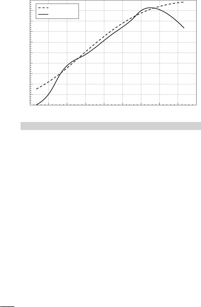
FIGURE 12.1

Predicted Probabilities of Positive Expenditure.

differ substantially. However, in this instance, the speciﬁcation tests are considerably more

sympathetic to the parametric model. Figure 12.1, which reproduces their Figure 2, compares

the predicted probabilities from the two models. The dashed curve is the probit model. Within

the range of most of the data, the models give quite similar predictions. Once again, however,

it is not possible to compare partial effects. The interesting outcome from this part of the

analysis seems to be that the failure of the parametric speciﬁcation resides more in the

modeling of the continuous expenditure variable than with the model that separates the two

subsamples based on zero or positive expenditures.

12.4 NONPARAMETRIC ESTIMATION

Researchers have long held reservations about the strong assumptions made in para-

metric models ﬁt by maximum likelihood. The linear regression model with normal

disturbances is a leading example. Splines, translog models, and polynomials all repre-

sent attempts to generalize the functional form. Nonetheless, questions remain about

how much generality can be obtained with such approximations. The techniques of non-

parametric estimation discard essentially all ﬁxed assumptions about functional form

and distribution. Given their very limited structure, it follows that nonparametric spec-

iﬁcations rarely provide very precise inferences. The beneﬁt is that what information

is provided is extremely robust. The centerpiece of this set of techniques is the kernel

density estimator that we have used in the preceding examples. We will examine some

examples, then examine an application to a bivariate regression.

The set of literature in this area of econometrics is large and rapidly growing. Major references which

provide an applied and theoretical foundation are H¨ardle (1990), Pagan and Ullah (1999), and Li and Racine

(2007).

CHAPTER 12

✦

Estimation Frameworks in Econometrics

445

12.4.1 KERNEL DENSITY ESTIMATION

Sample statistics such as a mean, variance, and range give summary information about

the values that a random variable may take. But, they do not sufﬁce to show the distribu-

tion of values that the random variable takes, and these may be of interest as well. The

density of the variable is used for this purpose. A fully parametric approach to density

estimation begins with an assumption about the form of a distribution. Estimation of

the density is accomplished by estimation of the parameters of the distribution. To take

the canonical example, if we decide that a variable is generated by a normal distribution

with mean μ and variance σ

, then the density is fully characterized by these parameters.

It follows that

f (x) = f (x | ˆμ, ˆσ

) =

ˆσ

√

2π

exp



−



x − ˆμ

ˆσ





One may be unwilling to make a narrow distributional assumption about the density.

The usual approach in this case is to begin with a histogram as a descriptive device.

Consider an example. In Examples 15.17 and in Greene (2004a), we estimate a model

that produces a conditional estimator of a slope vector for each of the 1,270 ﬁrms in

our sample. We might be interested in the distribution of these estimators across ﬁrms.

In particular, the conditional estimates of the estimated slope on ln sales for the 1,270

ﬁrms have a sample mean of 0.3428, a standard deviation of 0.08919, a minimum of

0.2361, and a maximum of 0.5664. This tells us little about the distribution of values,

though the fact that the mean is well below the midrange of 0.4013 might suggest some

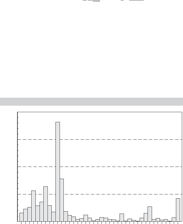
skewness. The histogram in Figure 12.2 is much more revealing. Based on what we see

FIGURE 12.2

Histogram for Estimated

sales

Coefﬁcients.

324

243

0.236 0.283 0.330 0.377 0.424

sales

0.471 0.518 0.565

Frequency

162

446

PART III

✦

Estimation Methodology

thus far, an assumption of normality might not be appropriate. The distribution seems

to be bimodal, but certainly no particular functional form seems natural.

The histogram is a crude density estimator. The rectangles in the ﬁgure are called

bins. By construction, they are of equal width. (The parameters of the histogram are

the number of bins, the bin width, and the leftmost starting point. Each is important

in the shape of the end result.) Because the frequency count in the bins sums to the

sample size, by dividing each by n, we have a density estimator that satisﬁes an obvious

requirement for a density; it sums (integrates) to one. We can formalize this by laying

out the method by which the frequencies are obtained. Let x

be the midpoint of the

kth bin and let h be the width of the bin—we will shortly rename h to be the bandwidth

for the density estimator. The distances to the left and right boundaries of the bins are

h/2. The frequency count in each bin is the number of observations in the sample which

fall in the range x

± h/2. Collecting terms, we have our “estimator”

f (x) =

frequency in bin

width of bin



i=1



x −

< x

< x +



where 1(statement) denotes an indicator function that equals 1 if the statement is true

and 0 if it is false and bin

denotes the bin which has x as its midpoint. We see, then, that

the histogram is an estimator, at least in some respects, like other estimators we have

encountered. The event in the indicator can be rearranged to produce an equivalent

form

f (x) =



i=1



−

− x



This form of the estimator simply counts the number of points that are within one

half-bin width of x

Albeit rather crude, this “naive” (its formal name in the literature) estimator is in

the form of kernel density estimators that we have met at various points;

f (x) =



i=1



− x



, where K[z] = 1[−1/2 < z < 1/2].

The naive estimator has several shortcomings. It is neither smooth nor continuous.

Its shape is partly determined by where the leftmost and rightmost terminals of the

histogram are set. (In constructing a histogram, one often chooses the bin width to be

a speciﬁed fraction of the sample range. If so, then the terminals of the lowest and

highest bins will equal the minimum and maximum values in the sample, and this will

partly determine the shape of the histogram. If, instead, the bin width is set irrespective

of the sample values, then this problem is resolved.) More importantly, the shape of

the histogram will be crucially dependent on the bandwidth itself. (Unfortunately, this

problem remains even with more sophisticated speciﬁcations.)

The crudeness of the weighting function in the estimator is easy to remedy. Rosen-

blatt’s (1956) suggestion was to substitute for the naive estimator some other weighting

function which is continuous and which also integrates to one. A number of candidates

have been suggested, including the (long) list in Table 12.1. Each of these is smooth,

continuous, symmetric, and equally attractive. The logit and normal kernels are deﬁned

so that the weight only asymptotically falls to zero whereas the others fall to zero at

CHAPTER 12

✦

Estimation Frameworks in Econometrics

447

TABLE 12.1

Kernels for Density Estimation

Kernel Formula K[z]

Epanechnikov 0.75(1 −0.2z

)/2.236 if |z|≤5, 0 else

Normal φ(z) (normal density),

Logit (z)[1 −(z)] (logistic density)

Uniform 0.5 if |z|≤1, 0 else

Beta 0.75(1 − z)(1 + z) if |z|≤1, 0 else

Cosine 1 +cos(2πz) if |z|≤0.5, 0 else

Triangle 1 −|z|,if |z|≤1, 0 else

Parzen 4/3 −8z

+ 8 |z|

if |z|≤0.5, 8(1 −|z|)

/3if0.5 < |z|≤1, 0 else.

speciﬁc points. It has been observed that in constructing a density estimator, the choice

of kernel function is rarely crucial, and is usually minor in importance compared to

the more difﬁcult problem of choosing the bandwidth. (The logit and normal kernels

appear to be the default choice in many applications.)

The kernel density function is an estimator. For any speciﬁc x,

f (x) is a sample

statistic,

f (z) =



i=1

g(x

|z, h).

Because g(x

|z, h) is nonlinear, we should expect a bias in a ﬁnite sample. It is tempting

to apply our usual results for sample moments, but the analysis is more complicated

because the bandwidth is a function of n. Pagan and Ullah (1999) have examined the

properties of kernel estimators in detail and found that under certain assumptions,

the estimator is consistent and asymptotically normally distributed but biased in ﬁnite

samples. The bias is a function of the bandwidth, but for an appropriate choice of h, the

bias does vanish asymptotically. As intuition might suggest, the larger is the bandwidth,

the greater is the bias, but at the same time, the smaller is the variance. This might suggest

a search for an optimal bandwidth. After a lengthy analysis of the subject, however, the

authors’ conclusion provides little guidance for ﬁnding one. One consideration does

seem useful. For the proportion of observations captured in the bin to converge to the

corresponding area under the density, the width itself must shrink more slowly than 1/n.

Common applications typically use a bandwidth equal to some multiple of n

−1/5

for this

reason. Thus, the one we used earlier is h = 0.9 × s/n

1/5

. To conclude the illustration

begun earlier, Figure 12.3 is a logit-based kernel density estimator for the distribution

of slope estimates for the model estimated earlier. The resemblance to the histogram

in Figure 12.2 is to be expected.

12.5 PROPERTIES OF ESTIMATORS

The preceding has been concerned with methods of estimation. We have surveyed a

variety of techniques that have appeared in the applied literature. We have not yet

examined the statistical properties of these estimators. Although, as noted earlier, we

will leave extensive analysis of the asymptotic theory for more advanced treatments, it

is appropriate to spend at least some time on the fundamental theoretical platform that

underlies these techniques.

448

PART III

✦

Estimation Methodology

0.2

0.00

0.3 0.4

sales

Density

0.5 0.6

7.20

5.76

4.32

2.88

1.44

FIGURE 12.3

Kernel Density for

sales

Coefﬁcients.

12.5.1 STATISTICAL PROPERTIES OF ESTIMATORS

Properties that we have considered are as follows:

•

Unbiasedness: This is a ﬁnite sample property that can be established in only a

very small number of cases. Strict unbiasedness is rarely of central importance

outside the linear regression model. However,“asymptotic unbiasedness” (whereby

the expectation of an estimator converges to the true parameter as the sample size

grows), might be of interest. [See, e.g., Pagan and Ullah (1999, Section 2.5.1 on the

subject of the kernel density estimator).] In most cases, however, discussions of

asymptotic unbiasedness are actually directed toward consistency, which is a more

desirable property.

•

Consistency: This is a much more important property. Econometricians are rarely

willing to place much credence in an estimator for which consistency cannot be

established.

•

Asymptotic normality: This property forms the platform for most of the statistical

inference that is done with common estimators. When asymptotic normality can-

not be established, it sometimes becomes difﬁcult to ﬁnd a method of progressing

beyond simple presentation of the numerical values of estimates (with caveats).

However, most of the contemporary literature in macroeconomics and time-series

analysis is strongly focused on estimators that are decidedly not asymptotically nor-

mally distributed. The implication is that this property takes its importance only in

context, not as an absolute virtue.

•

Asymptotic efﬁciency: Efﬁciency can rarely be established in absolute terms.

Efﬁciency within a class often can, however. Thus, for example, a great deal can

be said about the relative efﬁciency of maximum likelihood and GMM estimators