Greene W.H. Econometric Analysis

Подождите немного. Документ загружается.

MAXIMUM LIKELIHOOD

ESTIMATION

14.1 INTRODUCTION

The generalized method of moments discussed in Chapter 13 and the semiparametric,

nonparametric, and Bayesian estimators discussed in Chapters 12 and 16 are becoming

widely used by model builders. Nonetheless, the maximum likelihood estimator dis-

cussed in this chapter remains the preferred estimator in many more settings than the

others listed. As such, we focus our discussion of generally applied estimation methods

on this technique. Sections 14.2 through 14.6 present basic statistical results for estima-

tion and hypothesis testing based on the maximum likelihood principle. Sections 14.7

and 14.8 present two extensions of the method, two-step estimation and pseudo max-

imum likelihood estimation. After establishing the general results for this method of

estimation, we will then apply them to the more familiar setting of econometric mod-

els. The applications presented in Section 14.9 and 14.10 apply the maximum likelihood

method to most of the models in the preceding chapters and several others that illustrate

different uses of the technique.

14.2 THE LIKELIHOOD FUNCTION AND

IDENTIFICATION OF THE PARAMETERS

The probability density function, or pdf, for a random variable, y, conditioned on a

set of parameters, θ , is denoted f (y |θ ).

This function identiﬁes the data-generating

process that underlies an observed sample of data and, at the same time, provides a

mathematical description of the data that the process will produce. The joint density

of n independent and identically distributed (i.i.d.) observations from this process is the

product of the individual densities;

f (y

,...,y

|θ ) =

i=1

f (y

|θ ) = L(θ |y). (14-1)

This joint density is the likelihood function, deﬁned as a function of the unknown

parameter vector, θ, where y is used to indicate the collection of sample data. Note

that we write the joint density as a function of the data conditioned on the parameters

whereas when we form the likelihood function, we will write this function in reverse,

as a function of the parameters, conditioned on the data. Though the two functions are

the same, it is to be emphasized that the likelihood function is written in this fashion

Later we will extend this to the case of a random vector, y, with a multivariate density, but at this point, that

would complicate the notation without adding anything of substance to the discussion.

509

510

PART III

✦

Estimation Methodology

to highlight our interest in the parameters and the information about them that is

contained in the observed data. However, it is understood that the likelihood function

is not meant to represent a probability density for the parameters as it is in Chapter 16.

In this classical estimation framework, the parameters are assumed to be ﬁxed constants

that we hope to learn about from the data.

It is usually simpler to work with the log of the likelihood function:

ln L(θ |y) =



i=1

ln f (y

|θ ). (14-2)

Again, to emphasize our interest in the parameters, given the observed data, we denote

this function L(θ |data) = L(θ |y). The likelihood function and its logarithm, evalu-

ated at θ , are sometimes denoted simply L(θ) and ln L(θ), respectively, or, where no

ambiguity can arise, just L or ln L.

It will usually be necessary to generalize the concept of the likelihood function to

allow the density to depend on other conditioning variables. To jump immediately to

one of our central applications, suppose the disturbance in the classical linear regres-

sion model is normally distributed. Then, conditioned on its speciﬁc x

, y

is normally

distributed with mean μ



β and variance σ

. That means that the observed random

variables are not i.i.d.; they have different means. Nonetheless, the observations are

independent, and as we will examine in closer detail,

ln L(θ |y, X) =



i=1

ln f (y

, θ ) =−



i=1

[ln σ

+ ln(2π) + (y

− x



β)

/σ

], (14-3)

where X is the n × K matrix of data with ith row equal to x



The rest of this chapter will be concerned with obtaining estimates of the parameters,

θ, and in testing hypotheses about them and about the data-generating process. Before

we begin that study, we consider the question of whether estimation of the parameters

is possible at all—the question of identiﬁcation. Identiﬁcation is an issue related to the

formulation of the model. The issue of identiﬁcation must be resolved before estimation

can even be considered. The question posed is essentially this: Suppose we had an

inﬁnitely large sample—that is, for current purposes, all the information there is to be

had about the parameters. Could we uniquely determine the values of θ from such a

sample? As will be clear shortly, the answer is sometimes no.

DEFINITION 14.1

Identiﬁcation

The parameter vector θ is identiﬁed (estimable) if for any other parameter vector,

∗

= θ, for some data y, L(θ

∗

|y) = L(θ |y).

This result will be crucial at several points in what follows. We consider two examples,

the ﬁrst of which will be very familiar to you by now.

Example 14.1 Identiﬁcation of Parameters

For the regression model speciﬁed in (14-3), suppose that there is a nonzero vector a such

that x



a = 0 for every x

. Then there is another “parameter” vector, γ = β +a = β such that



β = x



γ for every x

. You can see in (14-3) that if this is the case, then the log-likelihood

CHAPTER 14

✦

Maximum Likelihood Estimation

511

is the same whether it is evaluated at β or at γ . As such, it is not possible to consider

estimation of β in this model because β cannot be distinguished from γ . This is the case of

perfect collinearity in the regression model, which we ruled out when we ﬁrst proposed the

linear regression model with “Assumption 2. Identiﬁability of the Model Parameters.”

The preceding dealt with a necessary characteristic of the sample data. We now consider

a model in which identiﬁcation is secured by the speciﬁcation of the parameters in the model.

(We will study this model in detail in Chapter 17.) Consider a simple form of the regression

model considered earlier, y

= β

+β

+ε

, where ε

has a normal distribution with zero

mean and variance σ

. To put the model in a context, consider a consumer’s purchases of

a large commodity such as a car where x

is the consumer’s income and y

is the difference

between what the consumer is willing to pay for the car, p

∗

, and the price tag on the car, p

Suppose rather than observing p

∗

or p

, we observe only whether the consumer actually

purchases the car, which, we assume, occurs when y

= p

∗

− p

is positive. Collecting this

information, our model states that they will purchase the car if y

> 0 and not purchase it if

≤ 0. Let us form the likelihood function for the observed data, which are purchase (or not)

and income. The random variable in this model is “purchase” or “not purchase”—there are

only two outcomes. The probability of a purchase is

Prob(purchase |β

, β

, σ, x

) = Prob( y

> 0 |β

, β

, σ, x

)

= Prob(β

+ β

+ ε

> 0 |β

, β

, σ, x

)

= Prob[ε

> −(β

+ β

) |β

, β

, σ, x

]

= Prob[ε

/σ > −(β

+ β

)/σ |β

, β

, σ, x

]

= Prob[z

> −(β

+ β

)/σ |β

, β

, σ, x

]

where z

has a standard normal distribution. The probability of not purchase is just one minus

this probability. The likelihood function is

i =purchased

[Prob(purchase |β

, β

, σ, x

)]

i =not purchased

[1 − Prob(purchase |β

, β

, σ, x

)].

We need go no further to see that the parameters of this model are not identiﬁed. If β

, β

, and

σ are all multiplied by the same nonzero constant, regardless of what it is, then Prob(purchase)

is unchanged, 1 − Prob(purchase) is also, and the likelihood function does not change. This

model requires a normalization. The one usually used is σ =1, but some authors [e.g.,

Horowitz (1993)] have used β

=1 instead.

14.3 EFFICIENT ESTIMATION: THE PRINCIPLE

OF MAXIMUM LIKELIHOOD

The principle of maximum likelihood provides a means of choosing an asymptotically

efﬁcient estimator for a parameter or a set of parameters. The logic of the technique is

easily illustrated in the setting of a discrete distribution. Consider a random sample of

the following 10 observations from a Poisson distribution: 5, 0, 1, 1, 0, 3, 2, 3, 4, and 1.

The density for each observation is

f (y

|θ) =

−θ

512

PART III

✦

Estimation Methodology

L(␪



x)  10

ln L(␪



x)  25

0.13

0.12

0.11

0.10

0.09

0.08

0.07

0.06

0.05

0.04

0.03

0.02

0.01

␪

3.53.22.92.62.32.01.71.41.10.8

0.50

ln L(␪



L(␪



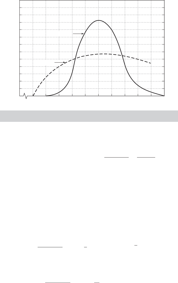
FIGURE 14.1

Likelihood and Log-Likelihood Functions for a Poisson

Distribution.

Because the observations are independent, their joint density, which is the likelihood

for this sample, is

f (y

, y

,...,y

|θ) =

i=1

f (y

|θ) =

−10θ



i=1

−10θ

207, 360

The last result gives the probability of observing this particular sample, assuming that a

Poisson distribution with as yet unknown parameter θ generated the data. What value

of θ would make this sample most probable? Figure 14.1 plots this function for various

values of θ. It has a single mode at θ =2, which would be the maximum likelihood

estimate, or MLE, of θ.

Consider maximizing L(θ |y) with respect to θ . Because the log function is mono-

tonically increasing and easier to work with, we usually maximize ln L(θ |y) instead; in

sampling from a Poisson population,

ln L(θ |y) =−nθ +ln θ



i=1

−



i=1

ln(y

!),

∂ ln L(θ |y)

∂θ

=−n +



i=1

= 0 ⇒

= y

For the assumed sample of observations,

ln L(θ |y) =−10θ + 20 ln θ − 12.242,

d ln L(θ |y)

dθ

=−10 +

= 0 ⇒

θ = 2,

CHAPTER 14

✦

Maximum Likelihood Estimation

513

and

ln L(θ |y)

dθ

−20

< 0 ⇒ this is a maximum.

The solution is the same as before. Figure 14.1 also plots the log of L(θ |y) to illustrate

the result.

The reference to the probability of observing the given sample is not exact in a

continuous distribution, because a particular sample has probability zero. Nonetheless,

the principle is the same. The values of the parameters that maximize L(θ |data) or its

log are the maximum likelihood estimates, denoted

θ. The logarithm is a monotonic

function, so the values that maximize L(θ |data) are the same as those that maximize

ln L(θ |data). The necessary condition for maximizing ln L(θ |data) is

∂ ln L(θ |data)

∂θ

= 0. (14-4)

This is called the likelihood equation. The general result then is that the MLE is a root

of the likelihood equation. The application to the parameters of the dgp for a discrete

random variable are suggestive that maximum likelihood is a “good” use of the data. It

remains to establish this as a general principle. We turn to that issue in the next section.

Example 14.2 Log-Likelihood Function and Likelihood Equations

for the Normal Distribution

In sampling from a normal distribution with mean μ and variance σ

, the log-likelihood func-

tion and the likelihood equations for μ and σ

are

ln L( μ, σ

) =−

ln(2π ) −

ln σ

−



i =1



( y

− μ)



, (14-5)

∂ ln L

∂μ



i =1

( y

− μ) = 0, (14-6)

∂ ln L

∂σ

=−

2σ



i =1

( y

− μ)

= 0. (14-7)

To solve the likelihood equations, multiply (14-6) by σ

and solve for ˆμ, then insert this solution

in (14-7) and solve for σ

. The solutions are

ˆμ



i =1

= y

and ˆσ



i =1

( y

− y

)

. (14-8)

14.4 PROPERTIES OF MAXIMUM LIKELIHOOD

ESTIMATORS

Maximum likelihood estimators (MLEs) are most attractive because of their large-

sample or asymptotic properties.

514

PART III

✦

Estimation Methodology

DEFINITION 14.2

Asymptotic Efﬁciency

An estimator is asymptotically efﬁcient if it is consistent, asymptotically normally

distributed (CAN), and has an asymptotic covariance matrix that is not larger than

the asymptotic covariance matrix of any other consistent, asymptotically normally

distributed estimator.

If certain regularity conditions are met, the MLE will have these properties. The ﬁnite

sample properties are sometimes less than optimal. For example, the MLE may be bi-

ased; the MLE of σ

in Example 14.2 is biased downward. The occasional statement that

the properties of the MLE are only optimal in large samples is not true, however. It can

be shown that when sampling is from an exponential family of distributions (see Deﬁni-

tion 13.1), there will exist sufﬁcient statistics. If so, MLEs will be functions of them, which

means that when minimum variance unbiased estimators exist, they will be MLEs. [See

Stuart and Ord (1989).] Most applications in econometrics do not involve exponential

families, so the appeal of the MLE remains primarily its asymptotic properties.

We use the following notation:

θ is the maximum likelihood estimator; θ

denotes

the true value of the parameter vector; θ denotes another possible value of the param-

eter vector, not the MLE and not necessarily the true values. Expectation based on the

true values of the parameters is denoted E

[.]. If we assume that the regularity condi-

tions discussed momentarily are met by f (x, θ

), then we have the following theorem.

THEOREM 14.1

Properties of an MLE

Under regularity, the maximum likelihood estimator (MLE) has the following

asymptotic properties:

M1. Consistency: plim

θ = θ

M2. Asymptotic normality:

∼ N[θ

, {I(θ

)}

−1

], where

I(θ

) =−E

[∂

ln L/∂θ

∂θ



M3. Asymptotic efﬁciency:

θ is asymptotically efﬁcient and achieves the Cram

er–

Rao lower bound for consistent estimators, given in M2 and Theorem C.2.

M4. Invariance: The maximum likelihood estimator of γ

= c(θ

) is c(

θ) if

c(θ

) is a continuous and continuously differentiable function.

14.4.1 REGULARITY CONDITIONS

To sketch proofs of these results, we ﬁrst obtain some useful properties of probability

density functions. We assume that (y

,...,y

) is a random sample from the population

with density function f (y

|θ

) and that the following regularity conditions hold. [Our

Not larger is deﬁned in the sense of (A-118): The covariance matrix of the less efﬁcient estimator equals that

of the efﬁcient estimator plus a nonnegative deﬁnite matrix.

CHAPTER 14

✦

Maximum Likelihood Estimation

515

statement of these is informal. A more rigorous treatment may be found in Stuart and

Ord (1989) or Davidson and MacKinnon (2004).]

DEFINITION 14.3

Regularity Conditions

R1. The ﬁrst three derivatives of ln f (y

|θ ) with respect to θ are continuous

and ﬁnite for almost all y

and for all θ. This condition ensures the existence

of a certain Taylor series approximation to and the ﬁnite variance of the

derivatives of ln L.

R2. The conditions necessary to obtain the expectations of the ﬁrst and second

derivatives of ln f (y

|θ ) are met.

R3. For all values of θ , |∂

ln f (y

|θ )/∂θ

∂θ

| is less than a function that

has a ﬁnite expectation. This condition will allow us to truncate the Taylor

series.

With these regularity conditions, we will obtain the following fundamental char-

acteristics of f (y

|θ ): D1 is simply a consequence of the deﬁnition of the likelihood

function. D2 leads to the moment condition which deﬁnes the maximum likelihood

estimator. On the one hand, the MLE is found as the maximizer of a function, which

mandates ﬁnding the vector that equates the gradient to zero. On the other, D2 is a

more fundamental relationship that places the MLE in the class of generalized method

of moments estimators. D3 produces what is known as the information matrix equality.

This relationship shows how to obtain the asymptotic covariance matrix of the MLE.

14.4.2 PROPERTIES OF REGULAR DENSITIES

Densities that are “regular” by Deﬁnition 14.3 have three properties that are used in

establishing the properties of maximum likelihood estimators:

THEOREM 14.2

Moments of the Derivatives of the Log-Likelihood

D1. ln f (y

|θ ), g

= ∂ ln f (y

|θ )/∂θ , and H

= ∂

ln f (y

|θ )/∂θ ∂θ



, i =

1,...,n, are all random samples of random variables. This statement fol-

lows from our assumption of random sampling. The notation g

(θ

) and

(θ

) indicates the derivative evaluated at θ

D2. E

(θ

)] = 0.

D3. Var[g

(θ

)] =−E [H

(θ

)].

Condition D1 is simply a consequence of the deﬁnition of the density.

For the moment, we allow the range of y

to depend on the parameters; A(θ

) ≤

≤ B(θ

). (Consider, for example, ﬁnding the maximum likelihood estimator of θ

for a continuous uniform distribution with range [0,θ

].) (In the following, the single

516

PART III

✦

Estimation Methodology

integral

...dy

, will be used to indicate the multiple integration over all the elements

of a multivariate of y

if that is necessary.) By deﬁnition,

B(θ

)

A(θ

)

f (y

|θ

) dy

= 1.

Now, differentiate this expression with respect to θ

. Leibnitz’s theorem gives

∂

B(θ

)

A(θ

)

f (y

|θ

) dy

∂θ

B(θ

)

A(θ

)

∂ f (y

|θ

)

∂θ

+ f (B(θ

) |θ

)

∂ B(θ

)

∂θ

− f (A(θ

) |θ

)

∂ A(θ

)

∂θ

= 0.

If the second and third terms go to zero, then we may interchange the operations of

differentiation and integration. The necessary condition is that lim

→A(θ

)

f (y

|θ

) =

lim

→B(θ

)

f (y

|θ

) = 0. (Note that the uniform distribution suggested earlier violates

this condition.) Sufﬁcient conditions are that the range of the observed random variable,

, does not depend on the parameters, which means that ∂ A(θ

)/∂θ

= ∂ B(θ

)/∂θ

= 0

or that the density is zero at the terminal points. This condition, then, is regularity

condition R2. The latter is usually assumed, and we will assume it in what follows. So,

∂

f (y

|θ

) dy

∂θ

∂ f (y

|θ

)

∂θ

∂ ln f (y

|θ

)

∂θ

f (y

|θ

) dy

= E



∂ ln f (y

|θ

)

∂θ



= 0.

This proves D2.

Because we may interchange the operations of integration and differentiation, we

differentiate under the integral once again to obtain



∂

ln f (y

|θ

)

∂θ



f (y

|θ

) +

∂ ln f (y

|θ

)

∂θ

∂ f (y

|θ

)

∂θ





= 0.

But

∂ f (y

|θ

)

∂θ



= f (y

|θ

)

∂ ln f (y

|θ

)

∂θ



and the integral of a sum is the sum of integrals. Therefore,

−



∂

ln f (y

|θ

)

∂θ





f (y

|θ

) dy



∂ ln f (y

|θ

)

∂θ

∂ ln f (y

|θ

)

∂θ





f (y

|θ

) dy

The left-hand side of the equation is the negative of the expected second derivatives

matrix. The right-hand side is the expected square (outer product) of the ﬁrst derivative

vector. But, because this vector has expected value 0 (we just showed this), the right-

hand side is the variance of the ﬁrst derivative vector, which proves D3:

Var



∂ ln f (y

|θ

)

∂θ



= E



∂ ln f (y

|θ

)

∂θ



∂ ln f (y

|θ

)

∂θ





=−E



∂

ln f (y

|θ

)

∂θ





CHAPTER 14

✦

Maximum Likelihood Estimation

517

14.4.3 THE LIKELIHOOD EQUATION

The log-likelihood function is

ln L(θ |y) =



i=1

ln f (y

|θ ).

The ﬁrst derivative vector, or score vector,is

g =

∂ ln L(θ |y)

∂θ



i=1

∂ ln f (y

|θ )

∂θ



i=1

. (14-9)

Because we are just adding terms, it follows from D1 and D2 that at θ



∂ ln L(θ

|y)

∂θ



= E

] = 0. (14-10)

which is the likelihood equation mentioned earlier.

14.4.4 THE INFORMATION MATRIX EQUALITY

The Hessian of the log-likelihood is

H =

∂

ln L(θ |y)

∂θ ∂θ





i=1

∂

ln f (y

|θ )

∂θ ∂θ





i=1

Evaluating once again at θ

, by taking



] = E

⎡

⎣



i=1



j=1



0 j

⎤

⎦

and, because of D1, dropping terms with unequal subscripts we obtain



] = E





i=1





= E





i=1

(−H

)



=−E

so that

Var



∂ ln L(θ

|y)

∂θ



= E



∂ ln L(θ

|y)

∂θ



∂ ln L(θ

|y)

∂θ





=−E



∂

ln L(θ

|y)

∂θ





(14-11)

This very useful result is known as the information matrix equality.

14.4.5 ASYMPTOTIC PROPERTIES OF THE MAXIMUM

LIKELIHOOD ESTIMATOR

We can now sketch a derivation of the asymptotic properties of the MLE. Formal proofs

of these results require some fairly intricate mathematics. Two widely cited derivations

are those of Cram´er (1948) and Amemiya (1985). To suggest the ﬂavor of the exercise,

we will sketch an analysis provided by Stuart and Ord (1989) for a simple case, and

indicate where it will be necessary to extend the derivation if it were to be fully general.

518

PART III

✦

Estimation Methodology

14.4.5.a Consistency

We assume that f (y

|θ

) is a possibly multivariate density that at this point does not

depend on covariates, x

. Thus, this is the i.i.d., random sampling case. Because

θ is the

MLE, in any ﬁnite sample, for any θ =

θ (including the true θ

) it must be true that

ln L(

θ) ≥ ln L(θ). (14-12)

Consider, then, the random variable L(θ)/L(θ

). Because the log function is strictly

concave, from Jensen’s Inequality (Theorem D.13.), we have



L(θ )

L(θ

)



< ln E



L(θ )

L(θ

)



. (14-13)

The expectation on the right-hand side is exactly equal to one, as



L(θ )

L(θ

)





L(θ )

L(θ

)



L(θ

) dy = 1 (14-14)

is simply the integral of a joint density. So, the right hand side of (14-13) equals zero.

Divide the left hand side of (14-13) by n to produce

[1/n ln L(θ)] − E

[1/n ln L(θ

)] < 0.

This produces a central result:

THEOREM 14.3

Likelihood Inequality

[(1/n) ln L(θ

)] > E

[(1/n) ln L(θ)] for any θ = θ

(including

θ).

In words, the expected value of the log-likelihood is maximized at the true value of the

parameters.

For any θ , including

θ,

[(1/n) ln L(θ)] = (1/n)



i=1

ln f (y

|θ )

is the sample mean of n i.i.d. random variables, with expectation E

[(1/n) ln L(θ)].

Because the sampling is i.i.d. by the regularity conditions, we can invoke the

Khinchine theorem, D.5; the sample mean converges in probability to the popu-

lation mean. Using θ =

θ, it follows from Theorem 14.3 that as n →∞,

lim Prob{[(1/n) ln L(

θ)] < [(1/n) ln L(θ

)]}=1if

θ =θ

. But,

θ is the MLE, so for every

n, (1/n) ln L(

θ) ≥(1/n) ln L(θ

). The only way these can both be true is if (1/n) times

the sample log-likelihood evaluated at the MLE converges to the population expecta-

tion of (1/n) times the log-likelihood evaluated at the true parameters. There remains

one ﬁnal step. Does (1/n) ln L(

θ) → (1/n) ln L(θ

) imply that

θ → θ

? If there is a

single parameter and the likelihood function is one to one, then clearly so. For more

general cases, this requires a further characterization of the likelihood function. If the

likelihood is strictly continuous and twice differentiable, which we assumed in the reg-

ularity conditions, and if the parameters of the model are identiﬁed which we assumed

at the beginning of this discussion, then yes, it does, so we have the result.