Greene W.H. Econometric Analysis

Подождите немного. Документ загружается.

CHAPTER 19

✦

Limited Dependent Variables

889

college attendance and once without. Any individual is observed in only one of the two

states, so the pure measurement is impossible.

Accommodating these two problems forms the focal point of this enormous and

still growing literature. Rubin’s causal model (1974, 1978) provides a useful framework

for the analysis. Every individual in a population has a potential outcome, y and can be

exposed to the treatment, C. We will denote by C

the indicator whether or not the in-

dividual receives the treatment. Thus, the potential outcomes are y

|(C

= 1) = y

and

|(C

= 0) = y

.Theaverage treatment effect, averaged across the entire population is

ATE = E[y

− y

The compelling complication is that the individual will exist in only one of the two states,

so it is not possible to estimate ATE without further assumptions. More speciﬁcally, what

the researcher would prefer see is the average treatment effect on the treated,

ATET = E[y

− y

= 1]

and note that the second term is the missing counterfactual.

One of the major themes of the recent research is to devise robust methods of

estimation that do not rely heavily on fragile assumptions such as identiﬁcation by

functional form (e.g., relying on bivariate normality) and identiﬁcation by exclusion

restrictions (e.g., relying on basic instrumental variable estimators). This is a challenging

exercise—we have relied heavily on these assumptions in most of the work in this

book up to this point. For purposes of the general speciﬁcation, we will denote by x

the exogenous information that will be brought to bear on this estimation problem.

The vector x may (usually will) be a set of variables that will appear in a regression

model, but it is useful to think more generally than that and consider x rather to be an

information set. Certain minimal assumptions are necessary to make any headway at

all. The following appear at different points in the analysis.

Conditional independence: Receiving the treatment, C

, does not depend on the

outcome variable once the effect of x on the outcome is accounted for. If assignment to

the treatment group is completely random, then we would omit the effect of x in this

assumption. This assumption is extended for regression approaches with the conditional

mean assumption: E[y

, C

= 1] = E[y

, C

= 0] = E[y

|x]. This states that

the outcome in the untreated state does not affect the participation.

Distribution of potential outcomes: The model that is used for the outcomes is the

same for treated and nontreated, f (y |x, T = 1) = f (y |x, T = 0). In a regression

context, this would mean that the same regression applies in both states and that the

disturbance is uncorrelated with T, or that T is exogenous. This is a very strong as-

sumption that we will relax later. For the present, it removes one of the complica-

tions noted previously, so a step in the model-building exercise will be to relax this

assumption.

Overlap assumption: For any value of x, 0 < Prob(C

= 1 |x)<1. The strict inequal-

ity in this assumption means that for any x, the population will contain a mix of treated

and nontreated individuals. The usefulness of the overlap assumption is that with it, we

can expect to ﬁnd, for any treated individual, an individual who looks like them but is

not treated. This assumption will be useful for regression approaches.

890

PART IV

✦

Cross Sections, Panel Data, and Microeconometrics

The following sections will describe three major parts of the research agenda on

treatment effects: regression analysis with control functions in Section 19.6.1, propensity

score matching in Section 19.6.2, and regression discontinuity design in Section 19.6.3. A

fourth area, instrumental variable estimation, was developed in Chapter 8. As noted, this

is a huge and rapidly growing literature. For example, Imbens and Wooldridge’s (2009)

survey paper runs 85 pages and includes nearly 300 references, most of them since 2000.

Our purpose here is to provide some of the vocabulary and a superﬁcial introduction

to methods. The survey papers by Imbens and Wooldridge (2009) and Jones and Rice

(2010) provide greater detail. The conference volume by Millment, Smith, and Vytlacil

(2008) contains many theoretical contributions and empirical applications.

A Journal

of Business and Economic Statistics symposium [Angrist (2001)] raised many of the

important questions on whether and how it is possible to measure treatment effects.

19.6.1 REGRESSION ANALYSIS OF TREATMENT EFFECTS

The basic model of selectivity outlined earlier has been extended in an impressive variety

of directions. An interesting application that has found wide use is the measurement of

treatment effects and program effectiveness.

An earnings equation that accounts for the value of a college education is

earnings

= x



β + δC

+ ε

where C

is a dummy variable indicating whether or not the individual attended college.

The same format has been used in any number of other analyses of programs, experi-

ments, and treatments. The question is: Does δ measure the value of a college education

(assuming that the rest of the regression model is correctly speciﬁed)? The answer is

no if the typical individual who chooses to go to college would have relatively high

earnings whether or not he or she went to college. The problem is one of self-selection.

If our observation is correct, then least squares estimates of δ will actually overestimate

the treatment effect. The same observation applies to estimates of the treatment effects

in other settings in which the individuals themselves decide whether or not they will

receive the treatment.

To put this in a more familiar context, suppose that we model program participation

(e.g., whether or not the individual goes to college) as

∗

= w



γ + u

= 1ifC

∗

> 0, 0 otherwise.

We also suppose that, consistent with our previous conjecture, u

and ε

are correlated.

Coupled with our earnings equation, we ﬁnd that

E [y

= 1, x

, w

] = x



β + δ + E [ε

= 1, x

, w

]

= x



β + δ + ρσ

λ(−w



γ )

(19-34)

once again. [See (19-24).] Evidently, a viable strategy for estimating this model is to use

the two-step estimator discussed earlier. The net result will be a different estimate of δ

In the initial essay in the volume, Goldberger (2008) reproduces Goldberger (1972) in which the author

explores the endogeneity issue in detail with speciﬁc reference to the Head Start program of the 1960s.

CHAPTER 19

✦

Limited Dependent Variables

891

that will account for the self-selected nature of program participation. For nonpartici-

pants, the counterpart to (19-34) is

E [y

= 0, x

, w

] = x



β + ρσ



−φ(w



γ )

1 − (w



γ )



. (19-35)

The difference in expected earnings between participants and nonparticipants is, then,

E [y

= 1, x

, w

] − E [y

= 0, x

, w

] = δ + ρσ





(1 − 

)



. (19-36)

If the selectivity correction λ

is omitted from the least squares regression, then this

difference is what is estimated by the least squares coefﬁcient on the treatment dummy

variable. But because (by assumption) all terms are positive, we see that least squares

overestimates the treatment effect. Note, ﬁnally, that simply estimating separate equa-

tions for participants and nonparticipants does not solve the problem. In fact, doing

so would be equivalent to estimating the two regressions of Example 19.12 by least

squares, which, as we have seen, would lead to inconsistent estimates of both sets of

parameters.

To describe the problem created by selection on the unobservables, we will drop

the independence assumptions. The model with endogenous participation and different

outcome equations would be

∗

= w



γ + u

, C

= 1 if C

∗

> 0 and 0 otherwise,

= x



+ ε

= x



+ ε

It is useful to combine the second and third equations in

= C



+ ε

) + (1 − C

)(x



+ ε

), j = 0, 1.

We assume joint normality for the three disturbances;

⎛

⎝

⎞

⎠

∼ N

⎡

⎣

⎛

⎝

⎞

⎠

⎛

⎝

1 ρ

⎞

⎠

⎤

⎦

The variance in the participation equation is normalized to one for a binary outcome,

as described earlier (Section 17.2). Endogeneity of the participation is implied by the

nonzero values of the correlations ρ

and ρ

. The familiar problem of the missing coun-

terfactual appears here in our inability to estimate θ

. The data will never contain

information on both states simultaneously, so it will be impossible to estimate a co-

variance of y

and y

(conditioned on x

or otherwise). Thus, the parameter θ

is not

identiﬁed (estimable)—we normalize it to zero. The parameters of this model after the

two normalizations can be estimated by two-step least squares as suggested in Sec-

tion 19.5.3, or by full information maximum likelihood. The average treatment effect

on the treated would be

ATET = E[y

= 1, x

, w

] − E[y

= 1, x

, w

]

= x



(β

− β

) + (ρ

− ρ

)















892

PART IV

✦

Cross Sections, Panel Data, and Microeconometrics

[See (19-34).] If the treatment assignment is completely random, then ρ

= ρ

= 0, and

we are left with the ﬁrst term. But, of course, it is the nonrandomness of the treatment

assignment that brought us to this point. Finally, if the two coefﬁcient vectors differ only

in their constant terms, β

0,0

and β

1,0

, then we are left with the same δ that appears in

(19-36)—the ATET would be β

0,1

+ C

(β

1,0

− β

0,0

There are many variations of this model in the empirical literature. They have been

applied to the analysis of education,

the Head Start program,

and a host of other

settings.

This strand of literature is particularly important because the use of dummy

variable models to analyze treatment effects and program participation has a long

history in empirical economics. This analysis has called into question the interpretation

of a number of received studies.

19.6.1.a The Normality Assumption

Some research has cast some skepticism on the selection model based on the normal

distribution. [See Goldberger (1983) for an early salvo in this literature.] Among the

ﬁndings are that the parameter estimates are surprisingly sensitive to the distributional

assumption that underlies the model. Of course, this fact in itself does not invalidate the

normality assumption, but it does call its generality into question. On the other hand,

the received evidence is convincing that sample selection, in the abstract, raises serious

problems, distributional questions aside. The literature—for example, Duncan (1986b),

Manski (1989, 1990), and Heckman (1990)—has suggested some promising approaches

based on robust and nonparametric estimators. These approaches obviously have the

virtue of greater generality. Unfortunately, the cost is that they generally are quite

limited in the breadth of the models they can accommodate. That is, one might gain

the robustness of a nonparametric estimator at the cost of being unable to make use of

the rich set of accompanying variables usually present in the panels to which selectivity

models are often applied. For example, the nonparametric bounds approach of Manski

(1990) is deﬁned for two regressors. Other methods [e.g., Duncan (1986b)] allow more

elaborate speciﬁcations.

Recent research includes speciﬁc attempts to move away from the normality as-

sumption.

An example is Martins (2001), building on Newey (1991), which takes the

core speciﬁcation as given in (19-22) as the platform but constructs an alternative to the

assumption of bivariate normality. Martins’s speciﬁcation modiﬁes the Heckman model

by employing an equation of the form

E [y

= 1, x

, w

] = x



β + μ(w



γ )

where the latter “selectivity correction” is not the inverse Mills ratio, but some other

result from a different model. The correction term is estimated using Klein and Spady’s

(1993) semiparametric binary choice estimator. Whether the conditional mean in the

selected sample should even remain a linear index function remains to be settled. Not

surprisingly, Martins’s results, based on two-step least squares differ only slightly from

Willis and Rosen (1979).

Goldberger (1972, 2008).

A useful summary of the issues is Barnow, Cain, and Goldberger (1981). See, also, Imbens and Wooldridge

(2009).

Again, Angrist (2001) is an important contribution to this literature.

CHAPTER 19

✦

Limited Dependent Variables

893

the conventional results based on normality. This approach is arguably only a fairly

small step away from the tight parameterization of the Heckman model. Other non-

and semiparametric speciﬁcations, for example, Honor`e and Kyriazidou (1997, 2000)

represent more substantial departures from the normal model, but are much less op-

erational.

The upshot is that the issue remains unsettled. For better or worse, the

empirical literature on the subject continues to be dominated by Heckman’s original

model built around the joint normal distribution.

19.6.1.b Estimating the Effect of Treatment on the Treated

Consider a regression approach to analyzing treatment effects in a two-period setting,

= θ

+ x



β + γ C

+ u

+ ε

, t = 0, 1,

where C

is the treatment dummy variable and u

is the unobserved individual effect.

The setting is the pre- and posttreatment analysis of the sort considered in this section,

where we examine the impact of a job training program on post training earnings.

Because there are two periods, a natural approach to the analysis is to examine the

changes,

y

= (θ

− θ

) + γC

+ (x

)



β + ε

where C

= 1 for the treated and 0 for the nontreated individuals, and the ﬁrst differ-

ences eliminate the unobserved individual effects. In the absence of controls (regressors,

), or assuming that the controls are unchanged, the estimator of the effect of the treat-

ment will be

ˆγ = [

y |(C

= 1)] − [y |(C

= 0)],

which is the difference in differences estimator. This simpliﬁes the problem considerably

but has several shortcomings. Most important, by using the simple differences, we have

lost our ability to discern what induced the change, whether it was the program or

something else, presumably in x

Even without the normality assumption, the preceding regression approach is more

tightly structured than many are comfortable with. A considerable amount of research

has focused on what assumptions are needed to reach that model and whether they are

likely to be appropriate in a given setting.

The overall objective of the analysis of the

preceding two sections is to evaluate the effect of a treatment, C

, on the individual

treated. The implicit counterfactual is an observation on what the “response” (depen-

dent variable) of the treated individual would have been had they not been treated.

But, of course, an individual will be in one state or the other, not both. Denote by y

the random variable that is the outcome variable in the absence of the treatment and

by y

the outcome when the treatment has taken place. The average treatment effect,

This particular work considers selection in a “panel” (mainly two periods). But, the panel data setting for

sample selection models is more involved than a cross-section analysis. In a panel data set, the “selection” is

likely to be a decision at the beginning of Period 1 to be in the data set for all subsequent periods. As such,

something more intricate than the model we have considered here is called for.

A sampling of the more important parts of the literature on this issue includes Heckman (1992, 1997),

Imbens and Angrist (1994), Manski (1996), and Wooldridge (2002a, Chapter 18).

894

PART IV

✦

Cross Sections, Panel Data, and Microeconometrics

averaged over the entire population is

ATE = E[y

− y

This is the impact of the treatment on an individual drawn at random from the entire

population. However, the desired quantity is not necessarily the ATE, but the average

treatment effect on the treated, which would be

ATE |T = E[y

− y

|C = 1].

The difﬁculty of measuring this is, once again, the counterfactual, E[y

|C = 1]. Whether

these two measures will be the same is at the center of the much of the discussion

on this subject. If treatment is completely randomly assigned, then E[y

|C = 1] =

E[y

|C = 0] = E[y

|C = j], j = 0, 1. This means that with completely random

treatment assignment

ATE = E[y

|C = 1] − E[y

|C = 0].

To put this in our example, if college attendance were completely randomly distributed

throughout the population, then the impact of college attendance on income (neglecting

other covariates at this point) could be measured simply by averaging the incomes of

college attendees and subtracting the average income of nonattendees. The preceding

theory might work for the treatment “having brown eyes,” but it is unlikely to work

for college attendance. Not only is the college attendance treatment not randomly

distributed, but the treatment “assignment” is surely related to expectations about y

versus y

, and, at a minimum, y

itself. (College is expensive.) More generally, the

researcher faces the difﬁculty in calculating treatment effects that assignment to the

treatment might not be exogenous.

The control function approach that we used in (19-34)–(19-36) is used to account

for the endogeneity of the treatment assignment in the regression context. The very

speciﬁc assumptions of the bivariate normal distribution of the unobservables some-

what simpliﬁes the estimation, because they make explicit what control function (λ

)

is appropriate to use in the regression. As Wooldridge (2002a, p. 622) points out, how-

ever, the binary variable in the treatment effects regression represents simply an en-

dogenous variable in a linear equation, amenable to instrumental variable estimation

(assuming suitable instruments are available). Barnow, Cain, and Goldberger (1981)

proposed a two-stage least squares estimator, with instrumental variable equal to the

predicted probability from the probit treatment assignment model. This is slightly

less parametric than (19-36) because, in principle, its validity does not rely on joint nor-

mality of the disturbances. Wooldridge (2002a, pp. 621–633) discusses the underlying

assumptions.

19.6.2 PROPENSITY SCORE MATCHING

If the treatment assignment is “completely ignorable,” then, as noted, estimation of

the treatment effects is greatly simpliﬁed. Suppose, as well, that there are observable

variables that inﬂuence both the outcome and the treatment assignment. Suppose it

is possible to obtain pairs of individuals matched by a common x

, one with C

= 0,

the other with C

= 1. If done with a sufﬁcient number of pairs so as to average over

CHAPTER 19

✦

Limited Dependent Variables

895

the population of x

’s, then a matching estimator, the average value of (y

=, 1) −

= 0), would estimate E[y

−y

], which is what we seek. Of course, it is optimistic

to hope to ﬁnd a large sample of such matched pairs, both because the sample overall

is ﬁnite and because there may be many regressors, and the “cells” in the distribution

of x

are likely to be thinly populated. This will be worse when the regressors are

continuous, for example, with a “family income” variable. Rosenbaum and Rubin (1983)

and others

suggested, instead, matching on the propensity score, F(x

) = Prob(C

1 |x

). Individuals with similar propensity scores are paired and the average treatment

effect is then estimated by the differences in outcomes. Various strategies are suggested

by the authors for obtaining the necessary subsamples and for verifying the conditions

under which the procedures will be valid. [See, e.g., Becker and Ichino (2002) and

Greene (2007c).]

Example 19.15 Treatment Effects on Earnings

LaLonde (1986) analyzed the results of a labor market experiment, The National Supported

Work Demonstration, in which a group of disadvantaged workers lacking basic job skills

were given work experience and counseling in a sheltered environment. Qualiﬁed applicants

were assigned to training positions randomly. The treatment group received the beneﬁts of the

program. Those in the control group “were left to fend for themselves.” [The demonstration

was run in numerous cities in the mid-1970s. See LaLonde (1986, pp. 605–609) for details

on the NSW experiments.] The training period was 1976–1977; the outcome of interest for

the sample examined here was posttraining 1978 earnings. LaLonde reports a large variety

of estimates of the treatment effect, for different subgroups and using different estimation

methods. Nonparametric estimates for the group in our sample are roughly $900 for the

income increment in the posttraining year. (See LaLonde, p. 609.) Similar results are reported

from a two-step regression-based estimator similar to (19-34) to (19-36). (See LaLonde’s

footnote to Table 6, p. 616.)

LaLonde’s data are fairly well traveled, having been used in replications and extensions

in, for example, Dehejia and Wahba (1999), Becker and Ichino (2002), and Greene (2007b, c).

We have reestimated the matching estimates reported in Becker and Ichino. The data in the

ﬁle used there (and here) contain 2,490 control observations and 185 treatment observations

on the following variables:

t = treatment dummy variable,

age = age in years,

educ = education in years,

marr = dummy variable for married,

black = dummy variable for black,

hisp = dummy variable for Hispanic,

nodegree = dummy for no degree (not used),

re74 = real earnings in 1974,

re75 = real earnings in 1975,

re78 = real earnings in 1978,

Other important references in this literature are Becker and Ichino (1999), Dehejia and Wahba (1999),

LaLonde (1986), Heckman, Ichimura, and Todd (1997, 1998), Heckman, Ichimura, Smith, and Todd (1998),

Heckman, LaLonde, and Smith (1999), Heckman, Tobias, and Vytlacil (2003), and Heckman and Vytlacil

(2000).

896

PART IV

✦

Cross Sections, Panel Data, and Microeconometrics

Transformed variables added to the equation are

age

= age squared,

educ

= educ squared,

re74

= re74 squared,

re75

= re75 squared,

black74 = black times 1(re74 = 0) .

We also scaled all earnings variables by 10,000 before beginning the analysis. (See Appendix

Table F19.3. The data are downloaded from the Web site http://www.nber.org/%7Erdehejia/

nswdata.html. The two speciﬁc subsamples are in http://www.nber.org/%7Erdehejia//psid

controls.txt and http://www.nber.org/%7Erdehejia/nswre74 treated.txt.) (We note that

Becker and Ichino report they were unable to replicate Dehejia and Wahba’s results, al-

though they could come reasonably close. We, in turn, were not able to replicate either set

of results, though we, likewise, obtained quite similar results.)

The analysis proceeded as follows: A logit model in which the included variables were a

constant, age, age

, education, education

, marr, black, hisp, re74, re75, re742, re752, and

black74 was computed for the treatment assignment. The ﬁtted probabilities are used for the

propensity scores. By means of an iterative search, the range of propensity scores was parti-

tioned into eight regions within which, by a simple F test, the mean scores of the treatments

and controls were not statistically different. The partitioning is shown in Table 19.10. The

1,347 observations are all the treated observations and the 1,162 control observations are

those whose propensity scores fell within the range of the scores for the treated observations.

Within each interval, each treated observation is paired with a small number of the nearest

control observations. We found the average difference between treated observation and

control to equal $1,574.35. Becker and Ichino reported $1,537.94.

As an experiment, we reﬁt the propensity score equation using a probit model, retaining

the ﬁtted probabilities. We then used the two-step estimator described earlier to ﬁt (19-34)

and (19-35) using the entire sample. The estimates of δ, ρ, and σ were −1.01437, 0.35519,

1.38426). Using the results from the probit model, we averaged the result in (19-36) for the

entire sample, obtaining an estimated treatment effect of $1,476.30.

TABLE 19.10

Empirical Distribution of Propensity Scores

Percent Lower Upper

0–5 0.000591 0.000783 Sample size = 1,347

5–10 0.000787 0.001061 Average score = 0.137238

10–15 0.001065 0.001377 Std. Dev score = 0.274079

15–20 0.001378 0.001748

20–25 0.001760 0.002321 Lower Upper # Obs

25–30 0.002340 0.002956 1 0.000591 0.098016 1041

30–35 0.002974 0.004057 2 0.098016 0.195440 63

35–40 0.004059 0.005272 3 0.195440 0.390289 65

40–45 0.005278 0.007486 4 0.390289 0.585138 36

45–50 0.007557 0.010451 5 0.585138 0.779986 32

50–55 0.010563 0.014643 6 0.779986 0.877411 17

55–60 0.014686 0.022462 7 0.877411 0.926123 7

60–65 0.022621 0.035060 8 0.926123 0.974835 86

65–70 0.035075 0.051415

70–75 0.051415 0.076188

75–80 0.076376 0.134189

80–85 0.134238 0.320638

85–90 0.321233 0.616002

90–95 0.624407 0.949418

95–100 0.949418 0.974835

CHAPTER 19

✦

Limited Dependent Variables

897

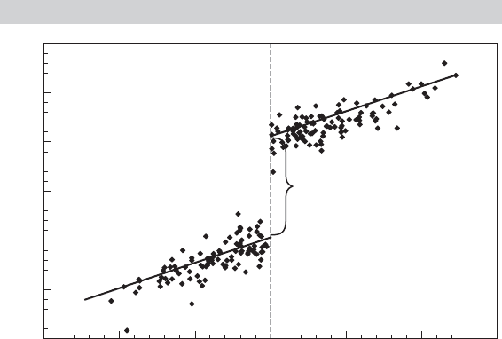
19.6.3 REGRESSION DISCONTINUITY

There are many situations in which there is no possibility of randomized assignment

of treatments. Examples include student outcomes and policy interventions in schools.

Angrist and Lavy (1999), for example, studied the effect of class sizes on test scores.

Van der Klaauw studied ﬁnancial aid offers that were tied to SAT scores and grade

point averages. In these cases, the natural experiment approach advocated by Angrist

and Pischke (2009) is an appealing way to proceed, when it is feasible. The regression

discontinuity design presents an alternative strategy. The conditions under which the

approach can be effective are when (1) the outcome, y, is a continuous variable; (2) the

outcome varies smoothly with an assignment variable, A, and (3) treatment is “sharply”

assigned based on the value of A, speciﬁcally C = 1(A > A

∗

) where A

∗

is a ﬁxed

threshold or cutoff value. [A “fuzzy design is based on Prob(C = 1 | A) = F( A).The

identiﬁcation problems with fuzzy design are much more complicated than with sharp

design. Readers are referred to Van der Klaauw (2002) for further discussion of fuzzy

design.] We assume, then, that

y = f (A, C) + ε.

Suppose, for example, the outcome variable is a test score, and that an administrative

treatment such as a special education program is funded based on the poverty rates of

certain communities. The ideal conditions for a regression discontinuity design based on

these assumptions is shown in Figure 19.8. The logic of the calculation is that the points

near the threshold value, which have “essentially” the same stimulus value, constitute

a nearly random sample of observations which are segmented by the treatment.

The method requires that E[ε | A, C] = E[ε | A]—the assignment variable—be ex-

ogenous to the experiment. The result in Figure 19.8 is consistent with

y = f (A) + αC + ε,

FIGURE 19.8

Regression Discontinuity.

Rate

RD Estimated

Treatment Effect

2 3 4 5 6 71

Score

898

PART IV

✦

Cross Sections, Panel Data, and Microeconometrics

where α will be the treatment effect to be estimated. The speciﬁcation of f (A) can be

problematic; assuming a linear function when something more general is appropriate

will bias the estimate of α. For this reason, nonparametric methods, such as the LOWESS

regression (see Section 12.3.5) might be attractive. This is likely to enable the analyst to

make fuller use of the observations that are more distant from the cutoff point. [See Van

der Klaaus (2002).] Identiﬁcation of the treatment effect begins with the assumption

that f ( A) is continuous at A

∗

, so that

lim

A↑A

∗

f (A) = lim

A↓A

∗

f (A) = f ( A

∗

Then

lim

A↓A

∗

E[y | A] − lim

A↑A

∗

E[y | A] = f ( A

∗

) + α + lim

A↓A

∗

E[ε | A] − f (A

∗

) − lim

A↑A

∗

E[ε | A]

= α.

With this in place, the treatment effect can be estimated by the difference of the average

outcomes for those individuals “close” to the threshold value, A

∗

. Details on regression

discontinuity design are provided by Trochim (1984, 2000) and Van der Klaauw (2002).

19.7 SUMMARY AND CONCLUSIONS

This chapter has examined settings in which, in principle, the linear regression model of

Chapter 2 would apply, but the data generating mechanism produces a nonlinear form:

truncation, censoring, and sample selection or endogenous sampling. For each case, we

develop the basic theory of the effect and then use the results in a major area of research

in econometrics.

In the truncated regression model, the range of the dependent variable is restricted

substantively. Certainly all economic data are restricted in this way—aggregate income

data cannot be negative, for example. But when data are truncated so that plausible

values of the dependent variable are precluded, for example, when zero values for ex-

penditure are discarded, the data that remain are analyzed with models that explicitly

account for the truncation. The stochastic frontier model is based on a composite dis-

turbance in which one part follows the assumptions of the familiar regression model

while the second component is built on a platform of the truncated regression.

When data are censored, values of the dependent variable that could in principle be

observed are masked. Ranges of values of the true variable being studied are observed

as a single value. The basic problem this presents for model building is that in such

a case, we observe variation of the independent variables without the corresponding

variation in the dependent variable that might be expected. Consistent estimation,

and useful interpretation of estimation results are based on maximum likelihood or

some other technique that explicitly accounts for the censoring mechanism. The most

common case of censoring in observed data arises in the context of duration analysis,

or survival functions (which borrows a term from medical statistics where this style

of model building originated). It is useful to think of duration, or survival data, as

the measurement of time between transitions or changes of state. We examined three

modeling approaches that correspond to the description in Chapter 12; nonparametric

(survival tables), semiparametric (the proportional hazard models), and parametric

(various forms such as the Weibull model).