Harris C.M., Piersol A.G. Harris Shock and vibration handbook

Подождите немного. Документ загружается.

identification of the standard(s) used in the calibration procedure. Depending on

the application, there may be one or more links to the national standard.

Primary and Secondary Standards. Primary standards,

6,7

maintained at national

metrology institutes, are derived from absolute measurements

of the transducer’s

sensitivity, measured in terms of seven basic units. For example, the absolute meas-

urement of “speed” must be made in terms of measurements of distance or distance

and time, not by a speedometer. Thus the word absolute implies nothing about preci-

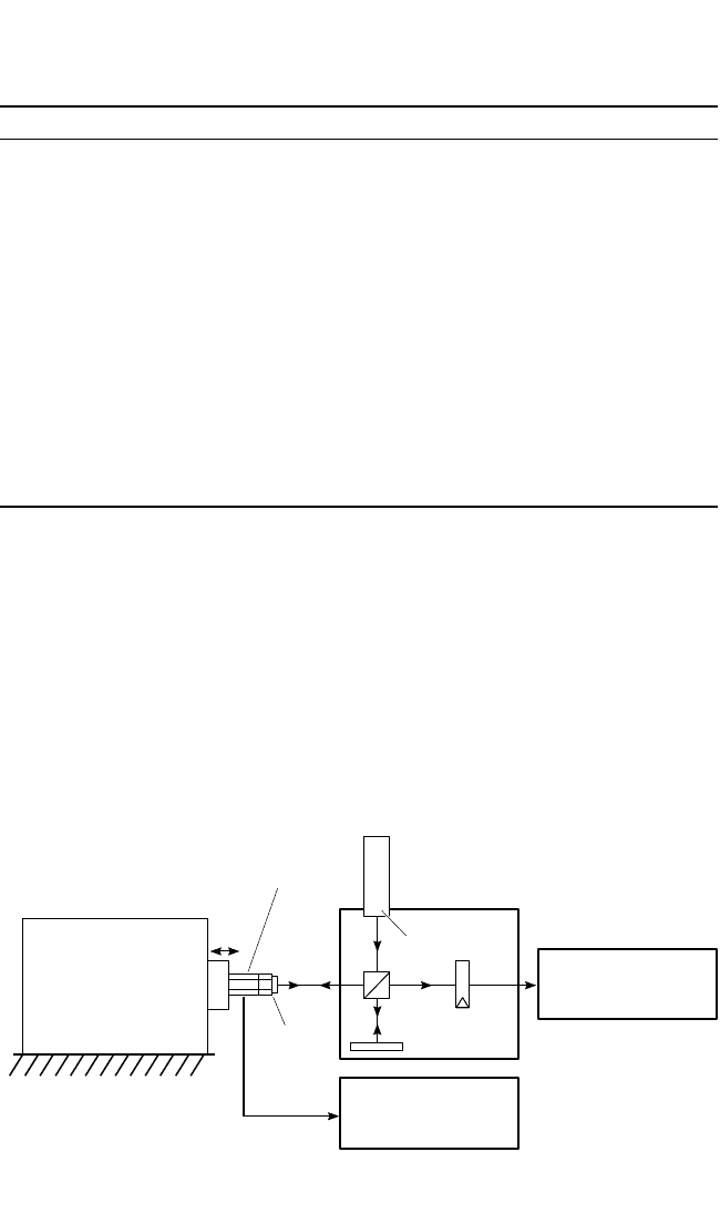
sion or accuracy. An example of a laboratory setup for the calibration of primary-

standard accelerometers, derived from absolute measurements, is shown in Fig.

18.2.

A vibration exciter generates sinusoidal motion which is measured by a

CALIBRATION OF PICKUPS 18.3

TABLE 18.1 National Standards Laboratories Responsible for the Calibration

of Vibration Pickups

Institution Laboratory Location Country

CSIRO Natl. Measurement Laboratory Lindfield Australia

INMETRO Laboratório de Vibrações Rio de Janeiro Brazil

NRC-CNRC Inst. Natl. Meas. Stds. Ottawa Canada

NIM Vibrations Laboratory Beijing China

CMU Primary Stds. of Kinematics Prague Czech Repub.

B&K Danish Prim. Lab. for Acoustics Naerum Denmark

BNM CEA/CESTA Belin-Beliet France

PTB Fachlabor. Beschleunigung Braunschweig Germany

IMGC Sezione Meccanica Torino Italy

NRLM Mechanical Metrology Dept. Tsukuba Japan

KSRI Division of Appl. Metrology Daedeog Danji Rep. of Korea

NMC SIRIM Berhad Malaysia

CENAM Div. Acustica y Vibraciones Queretaro Mexico

DSIR Measurement Stds. Laboratory Lower Hutt New Zealand

VNIIM Mendeleyev Inst. for Metrology St. Petersburg Russia

ITRI Center for Measurement Stds. Hsinchu Taiwan

NIST Manufacturing Metrology Div. Gaithersburg U.S.A.

AIRBORNE

ACCELERATION EXCITER

INTERFEROMETER

INDICATING

INSTRUMENT

(STANDARD)

SIGNAL-

PROCESSING

SYSTEM

DUMMY

MASS

LASER

LIGHT

DETECTOR

ACCELEROMETER

STANDARD

FIGURE 18.2 Primary (absolute) calibration of an accelerometer standard using laser interferom-

etry. (After von Martens.

)

8434_Harris_18_b.qxd 09/20/2001 12:13 PM Page 18.3

Michelson interferometer (described later in this chapter). The vibration is applied

to the base of the standard accelerometer whose output is measured. A dummy

mass, mounted on its top surface, simulates the conditions when this standard

accelerometer is used to calibrate a secondary standard

accelerometer by the com-

parison method described in the next section. Secondary standards (also referred to

as transfer standards or working standards) are maintained at various government

laboratories and industrial laboratories.A secondary standard accelerometer may be

calibrated either from absolute measurements or from a comparison with a primary

standard accelerometer. Such secondary standards are usually used for purposes of

comparisons of calibrations between laboratories or for checking production and

field units.

COMPARISON METHODS OF CALIBRATION

A rapid and convenient method of measuring the sensitivity of a vibration pickup to

be tested is by direct comparison of the pickup’s electrical output with that of a sec-

ond pickup (used as a “reference” standard) that has been calibrated by one of the

methods described in this chapter. A comparison method is used in most shock and

vibration laboratories, which periodically send their standards to a primary stan-

dards laboratory for recalibration. This procedure should be followed on a yearly

basis in order to establish a history of the accuracy and quality of its reference stan-

dard pickup.

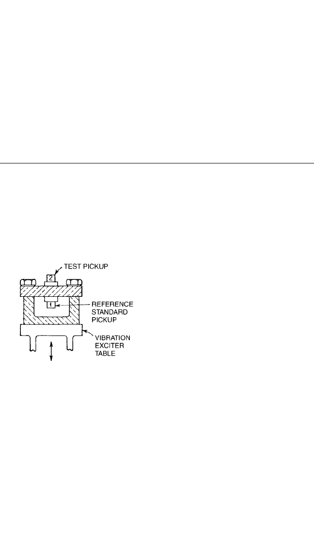
In this method of calibration the two

pickups usually are mounted back-to-

back on a vibration exciter as shown in

Fig. 18.3. It is essential to ensure that

each pickup experiences the same

motion. Any angular rotation of the

table should be small to avoid any dif-

ference in excitation between the two

pickup locations. The error due to rota-

tion may be reduced by carefully locat-

ing the pickups firmly on opposite faces

with the center-of-gravity of the pickups

located at the center of the table. Rela-

tive differences in pickup excitation may

be observed by reversing the pickup

locations and observing if the voltage

ratio is the same for both positions.

Calibration by the comparison method is limited to the range of frequencies and

amplitudes for which the reference standard pickup has been previously calibrated.

If both pickups are linear, the sensitivity of the test pickup can be calculated in both

magnitude and phase from

= S

(18.1)

where S

= sensitivity of test pickup

= sensitivity of reference standard pickup

= output voltage from test pickup

= output voltage from reference standard pickup



18.4 CHAPTER EIGHTEEN

FIGURE 18.3 Comparison method of calibra-

tion: Pickup 2 is calibrated against Pickup 1 (the

reference standard).The two pickups may be ex-

cited by any of the means described in this chap-

ter. (After ANSI Standard S2.2-1959, R 1997.

)

8434_Harris_18_b.qxd 09/20/2001 12:13 PM Page 18.4

Several calibration methods described below are variations on the implementation

of Eq. (18.1); they differ mainly in the manner of vibration excitation.

USING THE COMPARISON METHOD

A simple and convenient way of performing a comparison calibration is to fix the

test pickup and reference standard pickup so they experience identical motion, as in

Fig. 18.3.Then, set the frequency of the vibration exciter at a desired value, adjust the

amplitude of vibration of the vibration exciter to a desired value, and then compare

the electrical outputs of the pickups. Often, instead of making a comparison at a

fixed frequency, a graphical plot of the sensitivity versus frequency is obtained by

incorporating a swept-frequency signal generator in the calibration system.

RANDOM-EXCITATION-TRANSFER-FUNCTION METHOD

The use of random-vibration-excitation and transfer-function analysis techniques

can provide quick and accurate comparison calibrations.

The reference standard

pickup and the test pickup are mounted back-to-back on a suitable vibration exciter.

Their outputs are usually fed into a spectrum analyzer through a pair of low-pass

(antialiasing) filters. The bandwidth of the random signal which drives the exciter is

determined by settings of the analyzer.

This method provides a nearly continuous calibration over a desired frequency

spectrum, with the resulting sensitivity function having both amplitude and phase

information. Since purely sinusoidal motion is not a requirement as in the other cal-

ibration methods, this lessens the requirements for the power amplifier and exciter

to maintain low values of harmonic distortion. A very useful measure of process

quality is obtained by computing the input-output coherence function, which

requires knowledge of the input and output power spectra, the cross-power spec-

trum, and the transfer function.

CALIBRATION BY ABSOLUTE METHODS

RECIPROCITY METHOD

The reciprocity calibration method is an absolute means for calibrating vibration

exciters that have a velocity coil or reference accelerometer.This method relates the

pickup sensitivity to measurements of voltage ratio, resistance, frequency, and mass.

For this method to be applicable, it is necessary that the vibration exciter system be

linear (e.g., that the displacement, velocity, acceleration, and current in the driver

coil each increase linearly with force and driver-coil voltage). The reciprocity

method is used chiefly with electrodynamic exciters

but also with piezoelectric

vibration exciters.

The reciprocity method generally is applied only under controlled laboratory

conditions. Many precautions must be taken, and the process is usually time-

consuming. Several variations of the basic approach have been developed at

national standards laboratories.

14,15

The method described here has been used at the

CALIBRATION OF PICKUPS 18.5

8434_Harris_18_b.qxd 09/20/2001 12:13 PM Page 18.5

National Institute of Standards and Technology.

16–19

The method consists of two

laboratory experiments:

1. The measurement of the transfer admittance between the exciter’s driver coil

and the attached velocity coil or accelerometer.

2. The measurement of the voltage ratio of the open-circuit velocity coil or

accelerometer and the driving coil while the exciter is driven by a second exter-

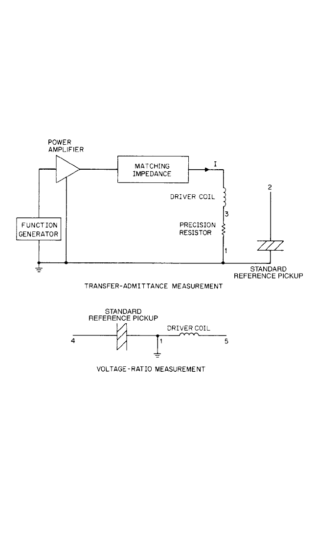
nal exciter.The use of a piezoelectric accelerometer is assumed here. The electri-

cal connections for the transfer admittance and voltage ratio measurements are

shown in Fig. 18.4.

18.6 CHAPTER EIGHTEEN

FIGURE 18.4 Transfer-admittance and voltage-ratio-measurement circuit connections

for the reciprocity calibration method in the Levy-Bouche realization.

The relationship defining the transfer admittance is

Y = (18.2)

where Y = transfer admittance

= voltage generated in standard accelerometer and amplifier

I = current in driver coil

and the bold letters denote phasor (complex) quantities.The current is determined by

measuring the voltage drop across a standard resistor.The phase,ψ

, of Y is measured

with a phase meter having an uncertainty of 0.1° or better. Transfer admittance

measurements are made with a series of masses attached, one at a time, to the table



8434_Harris_18_b.qxd 09/20/2001 12:13 PM Page 18.6

of the exciter.Also, a zero-load transfer admittance measurement is made before and

after attaching each mass. This zero-load measurement is denoted by Y

. Using the

measured values of Y and Y

, graphs of the real and imaginary values of the ratio

= (18.3)

are plotted versus M

for each frequency, where M

is the value of the mass attached

to the table.The zero intercepts, J

and J

, of the resulting nominally straight lines and

their slopes, Q

and Q

, are computed by a weighted least-squares method.

The val-

ues of Y

used in the calculations are obtained by averaging the values of the Y

measurements before and after each measurement of Y using different masses.

These computed values are used in determining the sensitivity of the standard.

The ratio of two voltages, measured while the exciter is driven with an external

exciter, is given by

R = (18.4)

where e

= voltage generated in standard accelerometer and amplifier, and e

open-circuit voltage in driving coil.

After R, J

, J

, Q

, and Q

have been determined for a number of frequencies, f, the

sensitivity of the exciter is calculated from the following relationship:

S =



1/2



1 +



(18.5)

where j = unit imaginary vector

J = J

+ jJ

Q = Q

+ jQ

M =

The sensitivity of the exciter is, therefore, determined from the measured quantities

Q, J, T, and f and from the masses M

which are attached to the exciter table. The

sensitivity as computed from Eq. (18.5) has the units of volts per meter per second

squared if the values of the measurements are in the SI system. If the masses M

are

not in kilograms, appropriate conversion factors must be applied to the quantities J,

Q, and M. A commonly used engineering formula,

with the mass expressed in

pounds and the sensitivity in millivolts per g,is

S = 2635



1/2

(18.6)

which also assumes that MQ/J  1, a condition usually satisfied in practice but which

should be verified experimentally.The use of a computer greatly facilitates the appli-

cation of the reciprocity calibration process.

Assuming the errors to be uncorrelated, a typical estimate of uncertainty

expected from a reciprocity calibration method is ±0.5 percent in the frequency

range 100 to 1000 Hz. This is a twofold improvement over the earlier systems.

18,19

The critical component in a reciprocity-based calibration system is the vibration

exciter. Electrodynamic exciters utilizing an air bearing are generally superior to

other types, for this application.



J(Y − Y

)



1 − Q(Y − Y

)



j2πf



Y − Y

CALIBRATION OF PICKUPS 18.7

8434_Harris_18_b.qxd 09/20/2001 12:13 PM Page 18.7

CALIBRATION USING THE EARTH’S GRAVITATIONAL FIELD

The earth’s gravitational field provides a convenient means of applying a small con-

stant acceleration to a vibration pickup. It is particularly useful in calibrating

accelerometers whose frequency range extends down to 0 Hz. A 2g change in accel-

eration may be obtained by first aligning the sensitivity axis of the transducer in one

direction of the earth’s gravitational field, as shown in Fig. 15.5A, and then inverting

it so the sensitive axis is aligned in the opposite direction.This method of calibration

is particularly useful in field work.

Accelerations in the 1–10g range can be generated by several methods, which have

been largely replaced by the structural gravimetric calibrator described in the next sec-

tion. In the tilting-support calibrator

the pickup is fastened to one end of an arm

attached to a platform. The arm may be set at any angle between 0° and 180° relative

to the vertical, thus yielding different values of acceleration.The pendulum calibrator

generates transient accelerations as great as 10g for a duration of about one second. In

the rotating-table calibrator

20,21

the disk on which the test pickup is mounted rotates at

a uniform angular rate about a horizontal axis in such a way that the pickup’s axis of

sensitivity rotates in a vertical plane. This method makes it possible to obtain both the

static and dynamic responses of the pickup in the same test setup.

Structural-Gravimetric Calibration. This technique provides a simple, robust, and

low-cost method of calibrating pickups.

22,23

The structural-gravimetric-calibration (SGC)

method is applicable over a broad frequency range because it relies on a quartz force

transducer as the reference pickup and the behavior of the simplest of structures (i.e., a

mass behaving as a rigid body). It references the acceleration of gravity and allows the

measurement of sensitivity magnitude and phase. The results of calibration using this

method agree within a fraction of 1 percent with those obtained by laser interferometry

and reciprocity methods.The following steps are the procedure of SGC method:

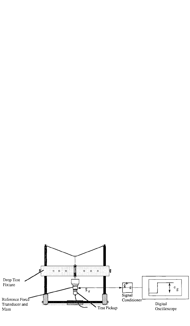
Step 1. Determine the acceleration sensitivity S

of the reference force transducer.

Mount the reference force transducer, reference mass (can be built-in or external),

and the test pickup to be calibrated on a drop-test fixture, as shown in Fig. 18.5. (For

use at higher frequencies it is important to make the reference mass small in size in

order to satisfy the rigid-body assumption.) Then subject the mass and the two pick-

ups to a free fall of 1g by striking the junction of line, which causes the line to relax

momentarily and impart a step-function gravitational acceleration to the assembly

by allowing it to fall freely. Measure the output of the reference force transducer, e

;

18.8 CHAPTER EIGHTEEN

FIGURE 18.5 Gravimetric free-fall calibrator for scaling reference force gage. (After D. Corelli

and R. W. Lally.

)

8434_Harris_18_b.qxd 09/20/2001 12:13 PM Page 18.8

in order to reduce the effect of measurement noise, curve fitting may be used to esti-

mate the step value. Equation (18.7) shows how the sensitivity of the reference force

transducer is related to the other parameters of the system.

 S

M  M  (18.7)

where S

= acceleration sensitivity of the reference force transducer, in mV/ms

2

= force sensitivity of the reference force transducer, in mV/N

M = total mass on the force transducer, in kg

= output of the force transducer, in mV

g = acceleration of free fall due to gravity, in ms

2

Note that e

is numerically equal to S

expressed in mV/g.

Step 2. Measure the voltage ratio e

. Remove the reference force transducer,

reference mass, and the pickup being calibrated from the drop-test fixture; then

mount them on the vibration exciter, as shown in Fig. 18.6. By measuring the trans-

fer function e

(i.e., the ratio of the voltage output of the signal conditioner from

the test pickup to the voltage output of the signal conditioner from the reference

force transducer, shown in Fig. 18.6) the frequency response of the test pickup can be



CALIBRATION OF PICKUPS 18.9

FIGURE 18.6 System configuration for frequency response calibration by measuring acceleration-

to-force ratio.

measured over 0.1 to 100,000 Hz, depending upon frequency range of the vibration

exciter and signal-to-noise ratio of the system. For use at low frequencies, the dis-

charge time constant of the reference force transducer should be ten times greater

than that of the test pickup.

Step 3. Calculate the sensitivity S

of the test pickup. If the reference force trans-

ducer and the test pickup are linear, the acceleration sensitivity of the test pickup S

expressed in the same units as S

, can be calculated from Eq. 18.1. If either velocity

or displacement sensitivity of the test pickup is required, it can be obtained by divid-

ing the acceleration sensitivity by 2f or (2f )

, respectively.

CENTRIFUGE CALIBRATOR

A centrifuge provides a convenient means of applying constant acceleration to a

pickup. Simple centrifuges can be obtained readily for acceleration levels up to 100g

8434_Harris_18_b.qxd 09/20/2001 12:13 PM Page 18.9

and can be custom-made for use at much higher values because of the light load

requirement by this application. They are particularly useful in calibrating rectilinear

accelerometers whose frequency range extends down to 0 Hz and whose sensitivity to

rotation is negligible. Centrifuges are mounted so as to rotate about a vertical axis.

Cable leads from the pickup, as well as power leads, usually are brought to the table

of the centrifuge through specially selected low-noise slip rings and brushes.

To perform a calibration, the accelerometer is mounted on the centrifuge with its

axis of sensitivity carefully aligned along a radius of the circle of rotation. If the cen-

trifuge rotates with an angular velocity of ω rad/sec, the acceleration a acting on the

pickup is

a =ω

r (18.8)

where r is the distance from the center-of-gravity of the mass element of the pickup

to the axis of rotation. If the exact location of the center-of-gravity of the mass in the

pickup is not known, the pickup is mounted with its positive sensing axis first out-

ward and then inward; then the average response is compared with the average

acceleration acting on the pickup as computed from Eq. (18.8) where r is taken as

the mean of the radii to a given point on the pickup case. The calibration factor is

determined by plotting the output e of the pickup as a function of the acceleration a

given by Eq. (18.8) for successive values of ω and then determining the slope of the

straight line fitted through the data.

INTERFEROMETER CALIBRATORS

A primary (absolute) method of calibrating an accelerometer using standard laser

interferometry is shown in Fig. 18.2. All systems in the following category of calibra-

tors consist of three stages: modulation, interference, and demodulation. The differ-

ences are in the specific type of interferometer that is used (for example, a

Michelson or Mach-Zehnder) and in the type of signal processing, which is usually

dictated by the nature of the vibration. The vibratory displacement to be measured

modulates one of the beams of the interferometer and is consequently encoded in

the output signal of the photodetector in both magnitude and phase.

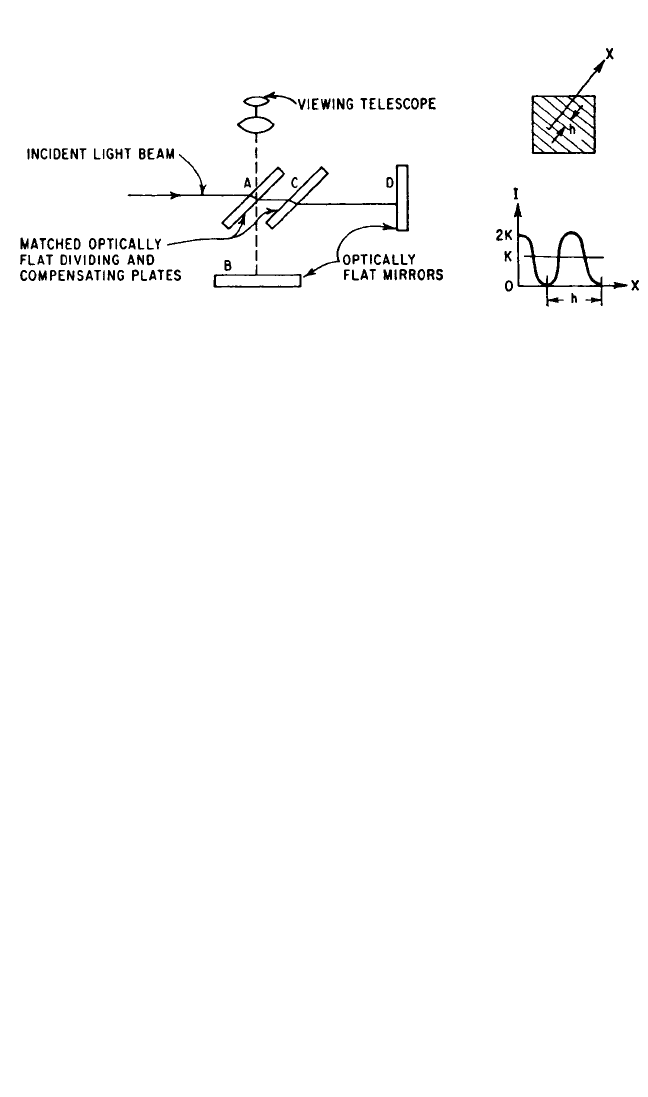
Figure 18.7 shows the principle of operation of the Michelson interferometer.

One of the mirrors, D in Fig. 18.7A, is attached to the plate on which the device to be

calibrated is mounted. Before exciting vibrations, it is necessary to obtain an inter-

ference pattern similar to that shown in Fig. 18.7B. The relationship underlying the

illustrations to be presented is the classical interference formula for the time aver-

age intensity I of the light impinging on the photodetector surface.

24,25

I = A + B cos 4πδ/λ (18.9)

where A and B are system constants depending on the transfer function of the detec-

tor, the intensities of the interfering beams, and alignment of the interferometer.The

vibration information is contained in the quantity δ,2δ being the optical-path differ-

ence of the interfering beams. The absoluteness of the measurement comes from λ,

the wavelength of the illumination, in terms of which the magnitude of vibratory dis-

placement is expressed. Velocity and acceleration values are obtained from dis-

placement measurements by differentiation with respect to time.

Fringe-Counting Interferometer. An optical interferometer is a natural instru-

ment for measuring vibration displacement.The Michelson and Fizeau interferome-

18.10 CHAPTER EIGHTEEN

8434_Harris_18_b.qxd 09/20/2001 12:13 PM Page 18.10

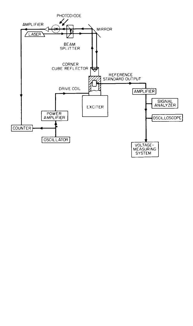
ters are the most popular configurations. A modified Michelson interferometer is

shown in Fig. 18.8.

A corner cube reflector is mounted on the vibration-exciter

table. A helium-neon laser is used as a source of illumination. The photodiode and

its amplifier must have sufficient bandwidth (as high as 10 MHz) to accommodate

the Doppler frequency shift associated with high velocities. An electrical pulse is

generated by the photodiode for each optical fringe passing it. The vibratory dis-

placement amplitude is directly proportional to the number of fringes per vibration

cycle. The peak acceleration can be calculated from

a = (18.10)

where λ=wavelength of light

ν=number of fringes per vibration cycle

f = vibration frequency

Interferometric fringe counting is useful for vibration-displacement measurement in

the lower frequency ranges, perhaps to several hundred hertz depending on the

characteristics of the vibration exciter.

27,28

At the low end of the frequency spectrum,

conventional procedures and commercially available equipment are not able to

meet all the present requirements. Low signal-to-noise ratios, cross-axis components

of motion, and zero-drifts are some of the problems usually encountered. In re-

sponse to those restrictions an electrodynamic exciter for the frequency range 0.01

to 20 Hz has been developed.

It features a maximum displacement amplitude of 0.5

meter, a transverse sensitivity less than 0.01 percent, and a maximum uncorrected

distortion of 2 percent. These characteristics have been achieved by means of a spe-

cially designed air bearing, an electro-optic control, and a suitable foundation.

Figure 18.9 shows the main components of a computer-controlled low-frequency

calibration system which employs this exciter. Its functions are (1) generation of sinu-

soidal vibrations, (2) measurement of rms and peak values of voltage and charge, (3)

measurement of displacement magnitude and phase response, and (4) control of non-

linear distortion and zero correction for the moving element inside a tubelike mag-

net. Position of the moving element is measured by a fringe-counting interferometer.

Uncertainties in accelerometer calibrations using this system have been reduced to

about 0.25 to 0.5 percent, depending on frequency and vibration amplitude.

λνπ



CALIBRATION OF PICKUPS 18.11

FIGURE 18.7 The principle of operation of a Michelson interferometer: (A) Optical system.

(B) Observed interference pattern. (C) Variation of the light intensity along the X axis.

(A) (C)

(B)

8434_Harris_18_b.qxd 09/20/2001 12:13 PM Page 18.11

Fringe-Disappearance Interferometer. The phenomenon of the interference

band disappearance in an optical interferometer can be used to establish a precisely

known amplitude of motion. Figure 18.7 shows the principle of operation of the

Michelson interferometer employed in this technique. One of the mirrors D, in Fig.

18.7A, is attached to the mounting plate of the calibrator. Before exciting vibrations

it is necessary to obtain an interference pattern similar to that shown in Fig. 18.7B.

When the mirror D vibrates sinusoidally

with a frequency f and a peak dis-

placement amplitude d, the time average of the light intensity I at position x, meas-

ured from a point midway between two dark bands, is given by

I = A + BJ



cos



(18.11)

where J

= zero-order Bessel function of the first kind

A and B = constants of measuring system

h = distance between fringes, as shown in Fig. 18.11B and C

For certain values of the argument, the Bessel function of zero order is zero; then the

fringe pattern disappears and a constant illumination intensity A is present. Elec-

tronic methods for more precisely establishing the fringe disappearance value of the

vibratory displacement have been successfully used at the National Institute of Stan-

dards and Technology

17,31

and elsewhere. The latter method has been fully auto-

mated using a desktop computer.

The use of piezoelectric exciters is common for high-frequency calibration of

accelerometers.

They provide pistonlike motion of relatively high amplitude and

2πx



4πd



18.12 CHAPTER EIGHTEEN

FIGURE 18.8 Typical laboratory setup for interferometric measurement of vibratory

displacement by fringe counting. (After R. S. Koyanagi.

)

8434_Harris_18_b.qxd 09/20/2001 12:13 PM Page 18.12