Harris C.M., Piersol A.G. Harris Shock and vibration handbook
Подождите немного. Документ загружается.


trum. Impact signals have proven to be quite popular due to the freedom of apply-
ing the input with some form of an instrumented hammer. While the concept is
straightforward, the effective utilization of an impact signal is very involved.
14
Step relaxation. The step relaxation signal is a transient deterministic signal
which is formed by releasing a previously applied static input. The sample period
begins at the instant that the release occurs. This signal is normally generated by
the application of a static force through a cable. The cable is then cut or allowed
to release through a shear pin arrangement.
Pure random. The pure random signal is an ergodic, stationary random signal
which has a Gaussian probability distribution. In general, the signal contains all
frequencies (not just integer multiples of the FFT frequency increment), but it
may be filtered to include only information in a frequency band of interest. The
measured input spectrum of the pure random signal is altered by any impedance
mismatch between the system and the exciter.
Pseudo-random. The pseudo-random signal is an ergodic, stationary random
signal consisting only of integer multiples of the FFT frequency increment. The
frequency spectrum of this signal has a constant amplitude with random phase. If
sufficient time is allowed in the measurement procedure for any transient
response to the initiation of the signal to decay, the resultant input and response
histories are periodic with respect to the sample period. The number of averages
used in the measurement procedure is only a function of the reduction of the
variance error. In a noise-free environment, only one average may be necessary.
Periodic random. The periodic random signal is an ergodic, stationary random
signal consisting only of integer multiples of the FFT frequency increment. The
frequency spectrum of this signal has random amplitude and random phase dis-
tribution. Since a single history does not contain information at all frequencies, a
number of histories must be involved in the measurement process. For each aver-
age, an input history is created with random amplitude and random phase. The
system is excited with this input in a repetitive cycle until the transient response
to the change in excitation signal decays.The input and response histories should
then be periodic with respect to the sample period and are recorded as one aver-
age in the total process. With each new average, a new history, uncorrelated with
previous input signals, is generated, so that the resulting measurement is com-
pletely randomized.
Random transient (burst random). The random transient signal is neither a
completely transient deterministic signal nor a completely ergodic, stationary
random signal but contains properties of both signal types. The frequency spec-
trum of this signal has random amplitude and random phase distribution and
contains energy throughout the frequency spectrum.The difference between this
signal and the periodic random signal is that the random transient history is trun-
cated to zero after some percentage of the sample period (normally 50 to 80 per-
cent). The measurement procedure duplicates the periodic random procedure,
but without the need to wait for the transient response to decay. The point at
which the input history is truncated is chosen so that the response history decays
to zero within the sample period. Even for lightly damped systems, the response
history decays to zero very quickly because of the damping provided by the
exciter system trying to maintain the input at zero. This damping provided by the
exciter system is often overlooked in the analysis of the characteristics of this sig-
nal type. Since this measured input, although not part of the generated signal,
includes the variation of the input during the decay of the response history, the
EXPERIMENTAL MODAL ANALYSIS 21.37
8434_Harris_21_b.qxd 09/20/2001 12:08 PM Page 21.37

input and response histories are totally observable within the sample period and
the system damping is unaffected.
Increased Frequency Resolution. An increase in the frequency resolution of a
frequency response function affects measurement errors in several ways. Finer fre-
quency resolution allows more exact determination of the damped natural fre-
quency of each modal vector. The increased frequency resolution means that the
level of a broad-band signal is reduced.The most important benefit of increased fre-
quency resolution, though, is a reduction of the leakage error. Since the distortion of
the frequency response function due to leakage is a function of frequency spacing,
not frequency, the increase in frequency resolution reduces the true bandwidth of
the leakage error centered at each damped natural frequency. In order to increase
the frequency resolution, the total time per history must be increased in direct pro-
portion.The longer data acquisition time increases the variance error problem when
transient signals are utilized for input as well as emphasizing any nonstationary
problem with the data. The increase of frequency resolution often requires multiple
acquisition and/or processing of the histories in order to obtain an equivalent fre-
quency range. This increases the data storage and documentation overhead as well
as extending the total test time.
There are two approaches to increasing the frequency resolution of a frequency
response function.The first approach involves increasing the number of spectral lines
in a baseband measurement. The advantage of this approach is that no additional
hardware or software is required. However, FFT analyzers do not always have the
capability to alter the number of spectral lines used in the measurement. The second
approach involves the reduction of the bandwidth of the measurement while holding
the number of spectral lines constant. If the lower frequency limit of the bandwidth is
always zero, no additional hardware or software is required. Ideally, though, for an
arbitrary bandwidth, hardware and/or software to perform a frequency-shifted, or
digitally filtered, FFT is required.
The frequency-shifted FFT process for computing the frequency response func-
tion has additional characteristics pertinent to the reduction of errors. Primarily,
more accurate information can be obtained on weak spectral components if the
bandwidth is chosen to avoid strong spectral components.The out-of-band rejection
of the frequency-shifted FFT is better than that of most analog filters that are used
in a measurement procedure to attempt to achieve the same results. Additionally,
the precision of the resulting frequency response function is improved due to
processor gain inherent in the frequency-shifted FFT calculation procedure.
4–6
Weighting Functions. Weighting functions, or data windows, are probably the
most common approach to the reduction of the leakage error in the frequency
response function (see Chap. 14). While weighting functions are sometimes desir-
able and necessary to modify the frequency-domain effects of truncating a signal in
the time domain, they are too often utilized when one of the other approaches to
error reduction would give superior results. Averaging, selective excitation, and
increasing the frequency resolution all act to reduce the leakage error by eliminat-
ing the cause of the error. Weighting functions, on the other hand, attempt to com-
pensate for the leakage error after the data have already been digitized.
Windows alter, or compensate for, the frequency-domain characteristic associ-
ated with the truncation of data in the time domain. Essentially, again using the nar-
row bandpass filter analogy, windows alter the characteristics of the bandpass filters
that are applied to the data.This compensation for the leakage error causes an atten-
dant distortion of the frequency and phase information of the frequency response
21.38 CHAPTER TWENTY-ONE
8434_Harris_21_b.qxd 09/20/2001 12:08 PM Page 21.38

function, particularly in the case of closely spaced, lightly damped system poles. This
distortion is a direct function of the width of the main lobe and the size of the side
lobes of the spectrum of the weighting function.
4–7
MODAL PARAMETER ESTIMATION
Modal parameter estimation, or modal identification, is a special case of system
identification where the a priori model of the system is known to be in the form of
modal parameters. Modal parameters include the complex-valued modal frequen-
cies λ
r
, modal vectors {ψ
r
}, and modal scaling (modal mass or modal A).Additionally,
most algorithms estimate modal participation vectors {L
r
} and residue vectors {A
r
}
as part of the overall process.
Modal parameter estimation involves estimating the modal parameters of a
structural system from measured input-output data. Most modal parameter estima-
tion is based upon the measured data being the frequency response function or the
equivalent impulse-response function, typically found by inverse Fourier transform-
ing the frequency response function. Therefore, the form of the model used to
represent the experimental data is normally stated in a mathematical frequency
response function (FRF) model using temporal (time or frequency) and spatial
(input degree-of-freedom and output degree-of-freedom) information.
In general, modal parameters are considered to be global properties of the sys-
tem. The concept of global modal parameters simply means that there is only one
answer for each modal parameter and that the modal parameter estimation solution
procedure enforces this constraint. Every frequency response or impulse-response
function measurement theoretically contains the information that is represented by
the characteristic equation, the modal frequencies, and damping. If individual meas-
urements are treated as independent of one another in the solution procedure, there
is nothing to guarantee that a single set of modal frequencies and damping is gener-
ated. Likewise, if more than one reference is measured in the data set, redundant
estimates of the modal vectors can be made unless the solution procedure utilizes all
references in the estimation process simultaneously. Most of the current modal
parameter estimation algorithms estimate the modal frequencies and damping in a
global sense, but very few estimate the modal vectors in a global sense.
Since the modal parameter estimation process involves a greatly overdetermined
problem, the estimates of modal parameters resulting from different algorithms are
not the same as a result of differences in the modal model and model domain, dif-
ferences in how the algorithms use the data, differences in the way the data are
weighted or condensed, and differences in user expertise.
MODAL IDENTIFICATION CONCEPTS
The most common approach in modal identification involves using numerical tech-
niques to separate the contributions of individual modes of vibration in measure-
ments such as frequency response functions. The concept involves estimating the
individual single degree-of-freedom (SDOF) contributions to the multiple degree-
of-freedom (MDOF) measurement.
[H(ω)]
N
o
× N
i
=
n
r = 1
+ (21.60)
[A
r
*]
N
o
× N
i
jω−λ
r
*
[A
r
]
N
o
× N
i
jω−λ
r
EXPERIMENTAL MODAL ANALYSIS 21.39
8434_Harris_21_b.qxd 09/20/2001 12:08 PM Page 21.39
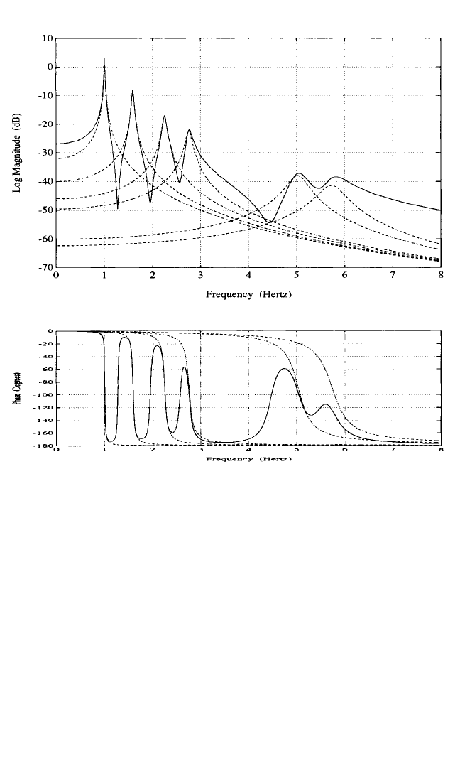
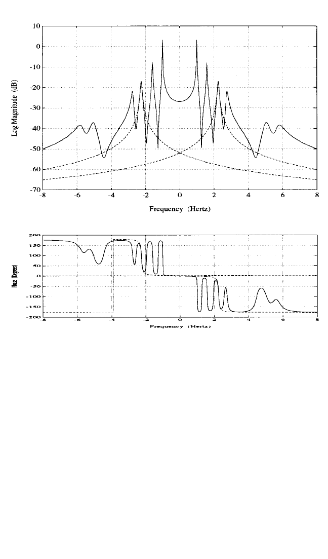
This concept is mathematically represented in Eq. (21.60) and graphically repre-
sented in Figs. 21.14 and 21.15.
Equation (21.60) is often formulated in terms of modal vectors {ψ
r
} and modal
participation vectors {L
r
} instead of residue matrices [A
r
]. Modal participation vec-
tors are a result of multiple reference modal parameter estimation algorithms and
relate how well each modal vector is excited from each of the reference locations
included in the measured data. The combination of the modal participation vector
{L
r
} and the modal vector {ψ
r
} for a given mode give the residue matrix A
pqr
= L
qr
ψ
pr
for that mode.
Generally, the modal parameter estimation process involves several stages. Typi-
cally, the modal frequencies and modal participation vectors are found in a first
stage and residues, modal vectors, and modal scaling are determined in a second
stage. Most modal parameter estimation algorithms can be reformulated into a sin-
gle, consistent mathematical formulation with a corresponding set of definitions and
unifying concepts.
15
Particularly, a matrix polynomial approach is used to unify the
presentation with respect to current algorithms such as the least squares complex
exponential (LSCE), polyreference time domain (PTD), Ibrahim time domain
(ITD), eigensystem realization algorithm (ERA), rational fraction polynomial
21.40 CHAPTER TWENTY-ONE
FIGURE 21.14 Modal superposition example (positive frequency poles).
8434_Harris_21_b.qxd 09/20/2001 12:08 PM Page 21.40
(RFP), polyreference frequency domain (PFD) and complex mode indication func-
tion (CMIF) methods. Using this unified matrix polynomial approach (UMPA)
allows a discussion of the similarities and differences of the commonly used methods
as well as a discussion of the numerical characteristics. Least squares (LS), total least
squares (TLS), double least squares (DLS), and singular value decomposition
(SVD) methods are used in order to take advantage of redundant measurement
data. Eigenvalue and singular value decomposition transformation methods are uti-
lized to reduce the effective size of the resulting eigenvalue-eigenvector problem as
well. Many acronyms used in modal parameter estimation are listed in Table 21.3.
Data Domain. Modal parameters can be estimated from a variety of different
measurements that exist as discrete data in different data domains (time, frequency,
and/or spatial). These measurements can include free decays, forced responses, fre-
quency responses, and unit impulse responses. These measurements can be
processed one at a time or in partial or complete sets simultaneously. The measure-
ments can be generated with no measured inputs, a single measured input, or multi-
ple measured inputs. The data can be measured individually or simultaneously. In
other words, there is a tremendous variation in the types of measurements and in the
EXPERIMENTAL MODAL ANALYSIS 21.41
FIGURE 21.15 Modal superposition example (positive and negative frequency poles).
8434_Harris_21_b.qxd 09/20/2001 12:09 PM Page 21.41

types of constraints that can be placed upon the testing procedures used to acquire
these data. For most measurement situations, frequency response functions are uti-
lized in the frequency domain and impulse-response functions are utilized in the
time domain.
Another important concept in experimental modal analysis, and particularly
modal parameter estimation, involves understanding the relationships between the
temporal (time and/or frequency) information and the spatial (input DOF and out-
put DOF) information. Input-output data measured on a structural system can
always be represented as a superposition of the underlying temporal characteristics
(modal frequencies) with the underlying spatial characteristics (modal vectors).
Model Order Relationships. The estimation of an appropriate model order is the
most important problem encountered in modal parameter estimation. This problem
is complicated because of the formulation of the parameter estimation model in the
time or frequency domain, a single or multiple reference formulation of the modal
parameter estimation model, and the effects of random and bias errors on the modal
parameter estimation model.The basis of the formulation of the correct model order
can be seen by expanding the theoretical second-order matrix equation of motion to
a higher-order model.
[m]s
2
+ [c]s + [k] =0 (21.61)
The above matrix polynomial is of model order two, has a matrix dimension of
n × n, and has a total of 2n characteristic roots (modal frequencies).This matrix poly-
nomial equation can be expanded to reduce the size of the matrices to a scalar equa-
tion.
α
2N
s
2N
+α
2N − 1
s
2N − 1
+α
2N − 2
s
2N − 2
+ ⋅⋅⋅ + α
0
= 0 (21.62)
The above matrix polynomial is of model order 2n, has a matrix dimension of
1 × 1, and has a total of 2n characteristic roots (modal frequencies). The characteris-
tic roots of this matrix polynomial equation are the same as those of the original
second-order matrix polynomial equation. Finally, the number of characteristic
21.42 CHAPTER TWENTY-ONE
TABLE 21.3 Modal Parameter Estimation Algorithm Acronyms
CEA Complex exponential algorithm
16
LSCE Least squares complex exponential
16
PTD Polyreference time domain
17, 18
ITD Ibrahim time domain
19
MRITD Multiple reference Ibrahim time domain
20
ERA Eigensystem realization algorithm
21, 22
PFD Polyreference frequency domain
23–25
SFD Simultaneous frequency domain
26
MRFD Multireference frequency domain
27
RFP Rational fraction polynomial
28
OP Orthogonal polynomial
29–31
CMIF Complex mode indication function
32
8434_Harris_21_b.qxd 09/20/2001 12:09 PM Page 21.42

roots (modal frequencies) that can be determined depends upon the size of the
matrix coefficients involved in the model and the order of the highest polynomial
term in the model.
For modal parameter estimation algorithms that utilize experimental data, the
matrix polynomial equations that are formed are a function of matrix dimension,
from 1 × 1 to N
i
× N
i
or N
o
× N
o
. There are a significant number of procedures that
have been formulated particularly for aiding in these decisions and selecting the
appropriate estimation model. Procedures for estimating the appropriate matrix
size and model order are another of the differences between various estimation
procedures.
Fundamental Measurement Models. Most current modal parameter estima-
tion algorithms utilize frequency- or impulse-response functions as the data, or
known information, to solve for modal parameters.The general equation that can be
used to represent the relationship between the measured frequency response func-
tion matrix and the modal parameters is shown in Eqs. (21.63) and (21.64).
[H(ω)]
N
o
× N
i
=
ψ
N
o
× 2N
2N × 2N
[L]
T
2N × N
i
(21.63)
[H(ω)]
T
N
i
× N
o
= [L]
N
i
× 2N
2N × 2N
ψ
T
2N × N
o
(21.64)
Impulse-response functions are rarely measured directly but are calculated from
associated frequency response functions via the inverse FFT algorithm.The general
equation that can be used to represent the relationship between the impulse-
response function matrix and the modal parameters is shown in Eqs. (21.9) and
(21.10).
[h(t)]
N
o
× N
i
=
ψ
N
o
× 2N
e
λ
r
t
2N × 2N
[L]
T
2N × N
i
(21.65)
[h(t)]
T
N
i
× N
o
= [L]
N
i
× 2N
e
λ
r
t
2N × 2N
ψ
T
2N × N
o
(21.66)
Many modal parameter estimation algorithms have been originally formulated
from Eqs. (21.63) through (21.66). However, a more general development for all
algorithms is based upon relating the above equations to a general matrix polyno-
mial approach.
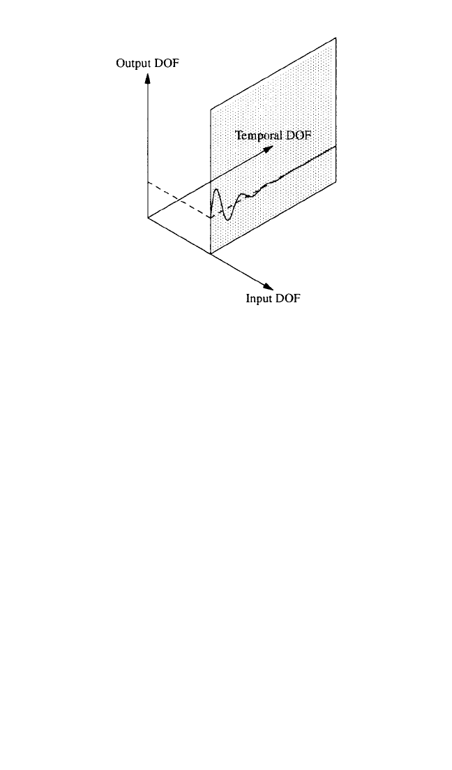
Characteristic Space. From a conceptual viewpoint, the measurement space of a
modal identification problem can be visualized as occupying a volume with the coor-
dinate axis defined in terms of three sets of characteristics.Two axes of the conceptual
volume correspond to spatial information and the third axis to temporal information.
The spatial coordinates are in terms of the input and output degrees-of-freedom
(DOF) of the system. The temporal axis is either time or frequency, depending upon
the domain of the measurements. These three axis define a 3-D volume which is
referred to as the characteristic space, as noted in Fig. 21.16.This space or volume rep-
1
jω−λ
r
1
jω−λ
r
EXPERIMENTAL MODAL ANALYSIS 21.43
8434_Harris_21_b.qxd 09/20/2001 12:09 PM Page 21.43
resents all possible measurement data as expressed by Eqs. (21.63) through (21.66).
This conceptual representation is very useful in understanding what data subspace
has been measured. Also, this conceptual representation is very useful in recognizing
how the data are organized and utilized with respect to different modal parameter
estimation algorithms. Information parallel to one of the axes consists of a solution
composed of the superposition of the characteristics defined by that axis. The other
two characteristics determine the scaling of each term in the superposition.
In modal parameter estimation algorithms that utilize a single frequency
response function, data collection is concentrated on measuring the temporal aspect
(time/frequency) at a sufficient resolution to determine the modal parameters. In
this approach, the accuracy of the modal parameters, particularly frequency and
damping, is essentially limited by Shannon’s sampling theorem and Rayleigh’s crite-
rion. This focus on the temporal information ignores the added accuracy that use of
the spatial information brings to the estimation of modal parameters. Recognizing
the characteristic space aspects of the measurement space and using these charac-
teristics (modal vector/participation vector) concepts in the solution procedure
leads to the conclusion that the spatial information can compensate for the limita-
tions of temporal information. Therefore, there is a tradeoff between temporal and
spatial information for a given accuracy requirement. This is particularly notable in
the case of repeated roots. No amount of temporal resolution (accuracy) can theo-
retically solve repeated roots, but the addition of spatial information in the form of
multiple inputs and/or outputs resolves this problem.
Any structural testing procedure measures a subspace of the total possible data
available. Modal parameter estimation algorithms may then use all of this subspace
or may choose to further limit the data to a more restrictive subspace. It is theoreti-
cally possible to estimate the characteristics of the total space by measuring a sub-
space which samples all three characteristics. However, the selection of the subspace
21.44 CHAPTER TWENTY-ONE
FIGURE 21.16 Conceptualization of modal
characteristic space (input DOF axis, output DOF
axis, time axis).
8434_Harris_21_b.qxd 09/20/2001 12:09 PM Page 21.44

has a significant influence on the results. In order for all of the modal parameters to
be estimated, the subspace must encompass a region which includes contributions of
all three characteristics.An important example is the necessity to use multiple refer-
ence data (inputs and outputs) in order to estimate repeated roots. The particular
subspace which is measured and the weighting of the data within the subspace in an
algorithm are the main differences among the various modal identification proce-
dures which have been developed.
In general, the amount of information in a measured subspace greatly exceeds
the amount necessary to solve for the unknown modal characteristics. Another
major difference among the various modal parameter estimation procedures is the
type of condensation algorithms that are used to reduce the data to match the num-
ber of unknowns [for example, least squares (LS), singular value decomposition
(SVD), etc.]. As is the case with any overspecified solution procedure, there is no
unique answer.The answer that is obtained depends upon the data that are selected,
the weighting of the data, and the unique algorithm used in the solution process. As
a result, the answer is the best answer depending upon the objective functions asso-
ciated with the algorithm being used. Historically, this point has created some con-
fusion since many users expect different methods to give exactly the same answer.
Many modal parameter estimation methods use information (subspace) where
only one or two characteristics are included. For example, the simplest (computa-
tionally) modal parameter estimation algorithms utilize one impulse-response func-
tion or one frequency response function at a time. In this case, only the temporal
characteristic is used, and, as might be expected, only temporal characteristics (modal
frequencies) can be estimated from the single measurement. The global characteris-
tic of modal frequency cannot be enforced. In practice, when multiple measurements
are taken, the modal frequency does not change from one measurement to the next.
Other modal parameter estimation algorithms utilize the data in a plane of the
characteristic space. For example, this corresponds to the data taken at a number of
response points but from a single excitation point or reference. This representation
of a column of measurements is shown in Fig. 21.16 as a plane in the characteristic
space. For this case, representing a single input (reference), while it is now possible
to enforce the global modal frequency assumption, it is not possible to compute
repeated roots and it is difficult to separate closely coupled modes because of the
lack of spatial data.
Many modal identification algorithms utilize data taken at a large number of out-
put DOFs due to excitation at a small number of input DOFs. Data taken in this
manner are consistent with a multiexciter type of test. Conceptually, this is repre-
sented by several planes of data parallel to the plane of data represented in Fig.
21.16. Some modal identification algorithms utilize data taken at a large number of
input DOFs and a small number of output DOFs. Data taken in this manner are con-
sistent with a roving hammer type of excitation with several fixed output sensors.
These data can also be generated by transposing the data matrix acquired using a
multiexciter test. The conceptual representation is several rows of the potential
measurement matrix perpendicular to the plane of data represented in Fig. 21.16.
Measurement data spaces involving many planes of measured data are the best pos-
sible modal identification situations, since the data subspace includes contributions
from temporal and spatial characteristics. This allows the best possibility of estimat-
ing all the important modal parameters. The data which define the subspace need to
be acquired through a consistent measurement process in order for the algorithms
to estimate accurate modal parameters. This means that the data must be measured
simultaneously and requires that data acquisition, digital signal processing, and
instrumentation be designed and operate accordingly.
EXPERIMENTAL MODAL ANALYSIS 21.45
8434_Harris_21_b.qxd 09/20/2001 12:09 PM Page 21.45

Fundamental Modal Identification Models. The common characteristics of dif-
ferent modal parameter estimation algorithms can be more readily identified by
using a matrix polynomial model rather than using a physically based mathematical
model. One way of understanding the basis of this model can be developed from the
polynomial model used for the frequency response function.
H
pq
(ω) == (21.67)
This can be rewritten as
H
pq
(ω) ==
n
k = 0
β
k
( jω)
k
(21.68)
m
k = 0
α
k
( jω)
k
Further rearranging yields the following equation, which is linear in the unknown α
and β terms:
m
k = 0
α
k
( jω)
k
X
p
(ω) =
n
k = 0
β
k
( jω)
k
F
q
(ω) (21.69)
Noting that the response function X
p
can be replaced by the frequency response
function H
pq
if the force function F
q
is assumed to be unity, the above equation can
be restated as
m
k = 0
α
k
( jω)
k
H
pq
(ω) =
n
k = 0
β
k
( jω)
k
(21.70)
The above formulation is essentially a linear equation in terms of the unknown
coefficients α
k
and β
k
. The equation is valid at each frequency of the measured
frequency response function. Since, in the worst case, the number of unknowns is
m + n + 2, the unknown coefficients can theoretically be determined if the frequency
response function has m + n + 2 or more discrete frequencies. Practically, this is
always the case. Note that the total number of unknown coefficients (or coefficient
matrices) is actually m + n + 1 since one coefficient (or coefficient matrix) can be
assumed to be 1 (or the identity matrix).This is the case because the equation can be
divided, or normalized, by one of the unknown coefficients (or coefficient matrices).
Note that numerical problems can result if the equation is normalized by a coeffi-
cient (or coefficient matrix) that is close to zero. Normally, the coefficient α
0
(or the
coefficient matrix [α
0
]) is chosen as unity (or the identity matrix).
The previous models can be generalized to represent the general multiple
input/multiple output case as follows:
m
k = 0
[α
k
]( jω)
k
{X(ω)} =
n
k = 0
[β
k
]( jω)
k
{F(ω)} (21.71)
X
p
(ω)
F
q
(ω)
β
n
( jω)
n
+β
n − 1
( jω)
n − 1
+ ⋅⋅⋅ + β
1
( jω)
1
+β
0
( jω)
0
α
m
( jω)
m
+α
m − 1
( jω)
m − 1
+ ⋅⋅⋅ + α
1
( jω)
1
+α
0
( jω)
0
X
p
(ω)
F
q
(ω)
21.46 CHAPTER TWENTY-ONE
8434_Harris_21_b.qxd 09/20/2001 12:09 PM Page 21.46