Harris C.M., Piersol A.G. Harris Shock and vibration handbook
Подождите немного. Документ загружается.


Note that the size of the coefficient matrices [α
k
] and [β
k
] is normally N
i
× N
i
or N
o
×
N
o
when the equations are developed from experimental data. Rather than the basic
model being developed in terms of force and response information, the models can
be stated in terms of frequency response information. The response vector {X(ω)}
can be replaced by a vector of frequency response functions {H(ω)} where either the
input or the output is held fixed. The force vector {F(ω)} is then replaced by an inci-
dence matrix {R} of the same size which is composed of all zeros except for unity at
the position in the vector consistent with the driving point measurement (common
input and output DOF).
m
k = 0
( jω)
k
[α
k
]
{H(ω)} =
n
k = 0
( jω)
k
[β
k
]
{R} (21.72)
where
H
1q
(ω)0
H
2q
(ω)0
H
3q
(ω)0
{H(ω)} =
...
{R} =
...
H
qq
(ω)1
... ...
H
pq
(ω)0
The above model, in the frequency domain, corresponds to an autoregressive
moving-average (ARMA) model that is developed from a set of finite difference
equations in the time domain. The general characteristic matrix polynomial model
concept recognizes that both the time- and frequency-domain models generate
essentially the same matrix polynomial models. For that reason, the unified matrix
polynomial approach (UMPA) terminology is used to describe both domains since
the ARMA terminology has been connected primarily with the time domain.
15
In parallel with the development of Eq. (21.67), a time-domain model represent-
ing the relationship between a single response degree-of-freedom and a single input
degree-of-freedom can be stated as follows:
m
k = 0
α
k
x(t
i + k
) =
n
k = 0
β
k
f(t
i + k
) (21.73)
For the general multiple input/multiple output case,
m
k = 0
[α
k
] {x(t
i + k
)} =
n
k = 0
[β
k
] {f(t
i + k
)} (21.74)
If the discussion is limited to the use of free decay or impulse-response function
data, the previous time-domain equations can be greatly simplified by noting that
the forcing function can be assumed to be zero for all time greater than zero. If this
is the case, the [β
k
] coefficients can be eliminated from the equations:
m
k = 0
[α
k
]
h
pq
(t
i + k
)
= 0 (21.75)
EXPERIMENTAL MODAL ANALYSIS 21.47
8434_Harris_21_b.qxd 09/20/2001 12:09 PM Page 21.47

In light of the above discussion, it is now apparent that most of the modal param-
eter estimation processes available can be developed by starting from a general
matrix polynomial formulation that is justifiable based upon the underlying matrix
differential equation. The general matrix polynomial formulation yields essentially
the same characteristic matrix polynomial equation for both time- and frequency-
domain data. For the frequency-domain data case, this yields
[α
m
] s
m
+ [α
m − 1
] s
m − 1
+ [α
m − 2
] s
m − 2
+ ⋅⋅⋅ + [α
0
] =0 (21.76)
For the time-domain data case, this yields
[α
m
] z
m
+ [α
m − 1
] z
m − 1
+ [α
m − 2
] z
m − 2
+ ⋅⋅⋅ + [α
0
] =0 (21.77)
With respect to the previous discussion of model order, the characteristic matrix
polynomial equation, Eq. (21.76) or (21.77), has a model order of m, and the number
of modal frequencies or roots that are found from this characteristic matrix polyno-
mial equation is m times the size of the coefficient matrices [α]. In terms of sampled
data, the time-domain matrix polynomial results from a set of finite difference equa-
tions and the frequency-domain matrix polynomial results from a set of linear equa-
tions, where each equation is formulated at one of the frequencies of the measured
data. This distinction is important to note since the roots of the matrix characteristic
equation formulated in the time domain are in the z domain (z
r
) and must be con-
verted to the frequency domain (λ
r
), while the roots of the matrix characteristic
equation formulated in the frequency domain (λ
r
) are already in the desired domain.
Note that the roots that are estimated in the time domain are limited to maximum
values determined by Shannon’s sampling theorem relationship (discrete time
steps).
z
r
= e
λ
r
∆t
λ
r
=σ
r
+ jω
r
(21.78)
σ
r
= Re
ω
r
= Im
Using this general formulation, the most commonly used modal identification meth-
ods can be summarized as shown in Table 21.4.
The high-order model is typically used for those cases where the system is under-
sampled in the spatial domain. For example, the limiting case is when only one meas-
urement is made on the structure. For this case, the left-hand side of the general
linear equation corresponds to a scalar polynomial equation with the order equal to
or greater than the number of desired modal frequencies. This type of high-order
model may yield significant numerical problems for the frequency-domain case.
The low-order model is used for those cases where the spatial information is
complete. In other words, the number of independent physical coordinates is greater
than the number of desired modal frequencies. For this case, the order of the left-
hand side of the general linear equation, Eq. (21.72) or (21.75), is equal to 1 or 2.
The zero-order model corresponds to a case where the temporal information is
neglected and only the spatial information is used. These methods directly estimate
the eigenvectors as a first step. In general, these methods are programmed to process
data at a single temporal condition or variable. In this case, the method is essentially
ln z
r
∆t
ln z
r
∆t
21.48 CHAPTER TWENTY-ONE
8434_Harris_21_b.qxd 09/20/2001 12:09 PM Page 21.48

equivalent to the single degree-of-freedom (SDOF) methods which have been used
with frequency response functions. In other words, the comparison between the
zeroth-order matrix polynomial model and the higher-order matrix polynomial
models is similar to the comparison between the SDOF and MDOF methods used
in modal parameter estimation.
Two-Stage Linear Solution Procedure. Almost all modal parameter estimation
algorithms in use at this time involve a two-stage linear solution approach. For
example, with respect to Eqs. (21.63) through (21.66), if all modal frequencies and
modal participation vectors can be found, the estimation of the complex residues
can proceed in a linear fashion. This procedure of separating the nonlinear problem
into a multistage linear problem is a common technique for most estimation meth-
ods today. For the case of structural dynamics, the common technique is to estimate
modal frequencies and modal participation vectors in a first stage and then to esti-
mate the modal coefficients plus any residuals in a second stage. Therefore, based
upon Eqs. (21.63) through (21.66), most commonly used modal identification algo-
rithms can be outlined as follows:
First stage of modal parameter estimation:
●
Load measured data into linear equation form [Eq. (21.72) or (21.75)].
●
Find scalar or matrix autoregressive coefficients [α
k
].
●
Normalize frequency range (frequency domain only).
●
Utilize orthogonal polynomials (frequency domain only).
●
Solve matrix polynomial for modal frequencies.
●
Formulate companion matrix.
●
Obtain eigenvalues of companion matrix λ
r
or z
r
.
●
Convert eigenvalues from z
r
to λ
r
(time domain only).
●
Obtain modal participation vectors L
qr
or modal vectors {ψ}
r
from eigenvec-
tors of the companion matrix.
Second stage of modal parameter estimation:
●
Find modal vectors and modal scaling from Eqs. (21.63) through (21.66).
EXPERIMENTAL MODAL ANALYSIS 21.49
TABLE 21.4 Characteristics of Modal Parameter Estimation Algorithms
Domain Matrix polynomial order Coefficients
Algorithm Time Frequency Zero Low High Scalar Matrix
CEA
● ●●
LSCE
● ●●
PTD
● ●
N
i
× N
i
ITD
●●
N
o
× N
o
MRITD
●●
N
o
× N
o
ERA
●●
N
o
× N
o
PFD
●●
N
o
× N
o
SFD
●●
N
o
× N
o
MRFD
●●
N
o
× N
o
RFP
●●●
Both
OP
●●●
Both
CMIF
●●
N
o
× N
i
8434_Harris_21_b.qxd 09/20/2001 12:09 PM Page 21.49
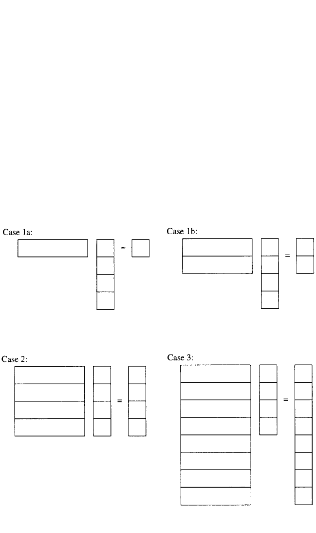
Equation (21.72) or (21.75) is used to formulate a single, block coefficient linear
equation as shown in the graphical analogy of Case 1a, Fig. 21.17. In order to esti-
mate complex conjugate pairs of roots, at least two equations from each piece or
block of data in the data space must be used. This situation is shown in Case 1b, Fig.
21.18. In order to develop enough equations to solve for the unknown matrix coeffi-
cients, further information is taken from the same block of data or from other blocks
of data in the data space until the number of equations equals (Case 2) or exceeds
(Case 3) the number of unknowns, as shown in Figs. 21.19 and 21.20. In the frequency
domain, this is accomplished by utilizing a different frequency from within each
measurement for each equation. In the time domain, this is accomplished by utiliz-
ing a different starting time or time shift from within each measurement for each
equation.
Once the matrix coefficients [α] have been found, the modal frequencies λ
r
or z
r
can be found using a number of numerical techniques.While in certain numerical sit-
uations, other numerical approaches may be more robust, a companion matrix
approach yields a consistent concept for understanding the process. Therefore, the
roots of the matrix characteristic equation can be found as the eigenvalues of the
associated companion matrix. The companion matrix can be formulated in one of
several ways. The most common formulation is as follows:
21.50 CHAPTER TWENTY-ONE
FIGURE 21.17 Underdetermined set of linear
equations.
FIGURE 21.18 Underdetermined set of lin-
ear equations.
FIGURE 21.19 Determined set of linear
equations.
FIGURE 21.20 Overdetermined set of linear
equations.
8434_Harris_21_b.qxd 09/20/2001 12:09 PM Page 21.50

−[α]
m − 1
−[α]
m − 2
... −[α]
1
−[α]
0
[I] [0] . . . [0] [0]
[0] [I] . . . [0] [0]
[0] [0] . . . [0] [0]
[C] =
... ... ... ... ...
(21.79)
[0] [0] . . . [0] [0]
[0] [0] . . . [0] [0]
[0] [0] . . . [I] [0]
Note again that the numerical characteristics of the eigenvalue solution of the com-
panion matrix are different for low-order cases than for high-order cases for a given
data set.The companion matrix can be used in the following eigenvalue formulation
to determine the modal frequencies for the original matrix coefficient equation:
[C]{X } =λ[I]{X } (21.80)
The eigenvectors that can be found from the eigenvalue-eigenvector solution uti-
lizing the companion matrix may or may not be useful in terms of modal parameters.
The eigenvector that is found, associated with each eigenvalue, is of length model
order times matrix coefficient size. In fact, the unique (meaningful) portion of the
eigenvector is of length equal to the size of the coefficient matrices and is repeated
in the eigenvector a model order number of times. Each time the unique portion of
the eigenvector is repeated, it is multiplied by a scalar multiple of the associated
modal frequency. Therefore, the eigenvectors of the companion matrix have the fol-
lowing form:
λ
r
m
{ψ}
r
⋅⋅⋅
{φ}
r
=
λ
r
2
{ψ}
r
(21.81)
λ
r
1
{ψ}
r
λ
r
0
{ψ}
r
r
Note that unless the size of the coefficient matrices is at least as large as the number
of measurement degrees-of-freedom, only a partial set of modal coefficients, the
modal participation coefficients L
qr
, are found. For the case involving scalar coeffi-
cients, no meaningful modal coefficients are found.
If the size of the coefficient matrices, and therefore the modal participation vector,
is less than the largest spatial dimension of the problem, then the modal vectors are
typically found in a second-stage solution process using one of Eqs. (21.63) through
(21.66). Even if the complete modal vector {ψ} of the system is found from the eigen-
vectors of the companion matrix approach, the modal scaling and modal participation
vectors for each modal frequency are normally found in this second-stage formulation.
EXPERIMENTAL MODAL ANALYSIS 21.51
8434_Harris_21_b.qxd 09/20/2001 12:09 PM Page 21.51

Data Sieving/Filtering. For almost all cases of modal identification, a large
amount of redundancy or overdetermination exists. This means that for Case 3,
defined in Fig. 21.20, the number of equations available compared to the number
required for the determined Case 2 (defined as the overdetermination factor) is quite
large. Beyond some value of overdetermination factor, the additional equations con-
tribute little to the result but may add significantly to the solution time. For this rea-
son, the data space is often filtered (limited in the temporal sense) or sieved (limited
in the input DOF or output DOF sense) in order to obtain a reasonable result in the
minimum time. For frequency-domain data, the filtering process normally involves
limiting the data set to a range of frequencies or a different frequency resolution
according to the desired frequency range of interest. For time-domain data, the fil-
tering process normally involves limiting the starting time value as well as the num-
ber of sets of time data taken from each measurement. Data sieving involves limiting
the data set to certain degrees-of-freedom that are of primary interest.This normally
involves restricting the data to specific directions (X, Y, and/or Z directions) or spe-
cific locations or groups of degrees-of-freedom, such as components of a large struc-
tural system.
Equation Condensation. Several important concepts should be delineated in
the area of equation condensation methods. Equation condensation methods are
used to reduce the number of equations based upon measured data to more closely
match the number of unknowns in the modal parameter estimation algorithms.
There are a large number of condensation algorithms available. Based upon the
modal parameter estimation algorithms in use today, the three types of algorithms
most often used are
●
Least squares. Least squares (LS), weighted least squares (WLS), total least
squares (TLS), or double least squares (DLS) methods are used to minimize the
squared error between the measured data and the estimation model. Historically,
this is one of the most popular procedures for finding a pseudo-inverse solution to
an overspecified system. The main advantage of this method is computational
speed and ease of implementation, while the major disadvantage is numerical pre-
cision.
●
Transformation. There are a large number of transformation that can be used to
reduce the data. In the transformation methods, the measured data are reduced by
approximating them by the superposition of a set of significant vectors. The num-
ber of significant vectors is equal to the amount of independent measured data.
This set of vectors is used to approximate the measured data and used as input to
the parameter estimation procedures. Singular value decomposition (SVD) is one
of the more popular transformation methods. The major advantage of such meth-
ods is numerical precision, and the disadvantage is computational speed and
memory requirements.
●
Coherent averaging. Coherent averaging is another popular method for reduc-
ing the data. In the coherent averaging method, the data are weighted by per-
forming a dot product between the data and a weighting vector (spatial filter).
Information in the data which is not coherent with the weighting vectors is aver-
aged out of the data. The method is often referred to as a spatial filtering proce-
dure. This method has both speed and precision but, in order to achieve precision,
requires a good set of weighting vectors. In general, the optimum weighting vec-
tors are connected with the solution, which is unknown. It should be noted that
least squares is an example of a noncoherent averaging process.
21.52 CHAPTER TWENTY-ONE
8434_Harris_21_b.qxd 09/20/2001 12:09 PM Page 21.52

The least squares and the transformation procedures tend to weight those modes
of vibration which are well excited. This can be a problem when trying to extract
modes which are not well excited.The solution is to use a weighting function for con-
densation which tends to enhance the mode of interest. This can be accomplished in
a number of ways:
●
In the time domain, a spatial filter or a coherent averaging process can be used to
filter the response to enhance a particular mode or set of modes. For example, by
averaging the data from two symmetric exciter locations, the symmetric modes of
vibration can be enhanced.A second example is to use only the data in a local area
of the system to enhance local modes. The third method is using estimates of the
modes’ shapes as weighting functions to enhance particular modes.
●
In the frequency domain, the data can be enhanced in the same manner as in the
time domain, plus the data can be additionally enhanced by weighting them in a
frequency band near the natural frequency of the mode of interest.
The type of equation condensation method that is utilized in a modal identifica-
tion algorithm has a significant influence on the results of the parameter estimation
process.
Coefficient Condensation. For the low-order modal identification algorithms, the
number of physical coordinates (typically N
o
) is often much larger than the number
of desired modal frequencies (2n). For this situation, the numerical solution proce-
dure is constrained to solve for N
o
or 2N
o
modal frequencies. This can be very time
consuming and is unnecessary.The number of physical coordinates N
o
can be reduced
to a more reasonable size (N
e
≈ N
o
or N
e
≈ 2N
o
) by using a decomposition transfor-
mation from physical coordinates N
o
to the approximate number of effective modal
frequencies N
e
. Currently, SVD or eigenvalue decompositions (ED) are used to pre-
serve the principal modal information prior to formulating the linear equation solu-
tion for unknown matrix coefficients.
33,34
In most cases, even when the spatial
information must be condensed, it is necessary to use a model order greater than 2 to
compensate for distortion errors or noise in the data and to compensate for the case
where the location of the transducers is not sufficient to totally define the structure.
[H′] = [T][H] (21.82)
where [H′] = transformed (condensed) frequency response function matrix
[T] = transformation matrix
[H] = original FRF matrix
The difference between the two techniques lies in the method of finding the trans-
formation matrix [T]. Once [H] has been condensed, however, the parameter esti-
mation procedure is the same as for the full data set. Because the data eliminated
from the parameter estimation process ideally correspond to the noise in the data,
the modal frequencies of the condensed data are the same as the modal frequencies
of the full data set. However, the modal vectors calculated from the condensed data
may need to be expanded back into the full space:
[Ψ] = [T]
T
[Ψ′] (21.83)
where [Ψ] = full-space modal matrix
[Ψ′] = condensed-space modal matrix
EXPERIMENTAL MODAL ANALYSIS 21.53
8434_Harris_21_b.qxd 09/20/2001 12:09 PM Page 21.53

Model Order Determination. Much of the work on modal parameter estimation
since 1975 has involved methodology for determining the correct model order for the
modal parameter model. Technically, model order refers to the highest power in
the matrix polynomial equation. The number of modal frequencies found is equal to
the model order times the size of the matrix coefficients, normally N
o
or N
i
. For a
given algorithm, the size of the matrix coefficients is normally fixed; therefore, deter-
mining the model order is directly linked to estimating n, the number of modal fre-
quencies in the measured data that are of interest. As has always been the case, an
estimate for the minimum number of modal frequencies can be easily found by
counting the number of peaks in the frequency response function in the frequency
band of analysis. This is a minimum estimate of n since the frequency response func-
tion measurement may be at a node of one or more modes of the system, repeated
roots may exist, and/or the frequency resolution of the measurement may be too
coarse to observe modes that are closely spaced in frequency. Several measurements
can be observed and a tabulation of peaks existing in any or all measurements can be
used as a more accurate minimum estimate of n. A more automated procedure for
including the peaks that are present in several frequency response functions is to
observe the summation of frequency response function power. This function repre-
sents the autopower or automoment of the frequency response functions summed
over a number of response measurements and is normally formulated as follows:
H
power
(ω) =
N
o
p = 1
N
i
q = 1
H
pq
(ω) H
pq
*(ω) (21.84)
These techniques are extremely useful but do not provide an accurate estimate of
model order when repeated roots exist or when modes are closely spaced in fre-
quency. For these reasons, an appropriate estimate of the order of the model is
of prime concern and is the single most important problem in modal parameter
estimation.
In order to determine a reasonable estimate of the model order for a set of rep-
resentative data, a number of techniques have been developed as guides or aids to
the user. Much of the user interaction involved in modal parameter estimation
involves the use of these tools. Most of the techniques that have been developed
allow the user to establish a maximum model order to be evaluated (in many cases,
this is set by the memory limits of the computer algorithm). Information is utilized
from the measured data based upon an assumption that the model order is equal to
this maximum. This information is evaluated in a sequential fashion to determine if
a model order less than the maximum is sufficient to describe the data sufficiently.
This is the point at which the user’s judgment and the use of various evaluation aids
becomes important. Some of the commonly used techniques are:
●
Measurement synthesis and comparison (curve-fit)
●
Error chart
●
Stability diagram
●
Mode indication functions
●
Rank estimation
One of the most common techniques is to synthesize an impulse-response func-
tion or a frequency response function and compare it to the measured function to
see if modes have been missed. This curve-fitting procedure is also used as a meas-
ure of the overall success of the modal parameter estimation procedure. The differ-
21.54 CHAPTER TWENTY-ONE
8434_Harris_21_b.qxd 09/20/2001 12:09 PM Page 21.54
ence between the two functions can be quantified and normalized to give an indica-
tor of the degree of fit. There can be many reasons for a poor comparison; incorrect
model order is one of the possibilities.
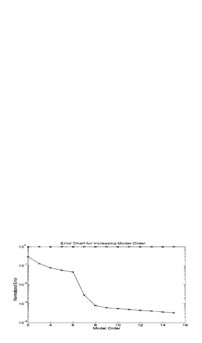
Error Chart. Another method that has been used to indicate the correct model
order more directly is the error chart. Essentially, the error chart is a plot of the error
in the model as a function of increasing model order.The error in the model is a nor-
malized quantity that represents the ability of the model to predict data that are not
involved in the estimate of the model parameters. For example, when measured data
in the form of an impulse-response function are used, only a small percentage of the
total number of data values are involved in the estimate of modal parameters. If the
model is estimated based upon 10 modes, only 4 × 10 data points are required, at a
minimum, to estimate the modal parameters if no additional spatial information is
used.The error in the model can then be estimated by the ability of the model to pre-
dict the next several data points in the impulse-response function compared to the
measured data points. For the case of 10 modes and 40 data points, the error in the
model is calculated from the predicted and measured data points 41 through 50.
When the model order is insufficient, this error is large, but when the model order
reaches the correct value, further increase in the model order does not result in a fur-
ther decrease in the error. Figure 21.21 is an example of an error chart.
Stability Diagram. A further enhancement of the error chart is the stability
diagram. The stability diagram is developed in the same fashion as the error chart
and involves tracking the estimates of frequency, damping, and possibly modal par-
ticipation factors as a function of model order.As the model order is increased, more
and more modal frequencies are estimated, but, hopefully, the estimates of the phys-
ical modal parameters stabilize as the correct model order is found. For modes that
are very active in the measured data, the modal parameters stabilize at a very low
model order. For modes that are poorly excited in the measured data, the modal
parameters may not stabilize until a very high model order is chosen. Nevertheless,
the nonphysical (computational) modes do not stabilize at all during this process
and can be sorted out of the modal parameter data set more easily. Note that incon-
sistencies (frequency shifts, leakage errors, etc.) in the measured data set obscure the
stability and make the stability diagram difficult to use. Normally, a tolerance, in per-
centage, is given for the stability of each of the modal parameters that are being eval-
uated. Figure 21.22 is an example of a stability diagram. In Fig. 21.22, a summation of
EXPERIMENTAL MODAL ANALYSIS 21.55
FIGURE 21.21 Model order determination: error chart.
8434_Harris_21_b.qxd 09/20/2001 12:09 PM Page 21.55
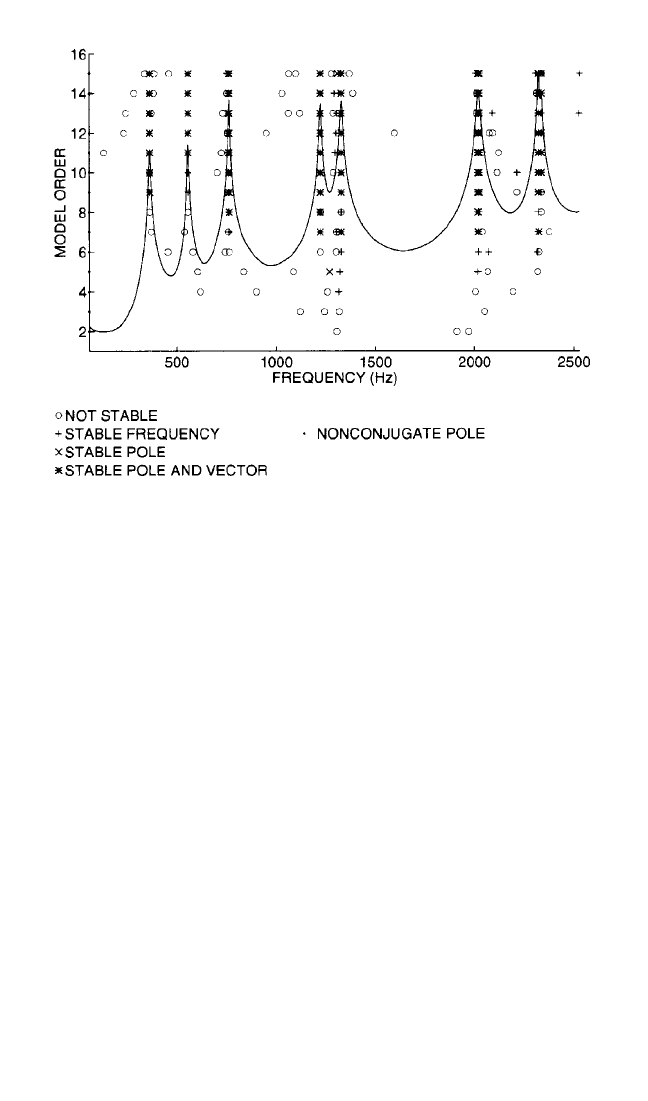
the frequency response function power is plotted on the stability diagram for refer-
ence. Other mode indication functions can also be plotted against the stability dia-
gram for reference.
Mode Indication Functions. Mode indication functions (MIF) are normally
real-valued, frequency-domain functions that exhibit local minima or maxima at the
modal frequencies of the system. One mode indication function can be plotted for
each reference available in the measured data. The primary mode indication func-
tion exhibits a local minimum or maximum at each of the natural frequencies of the
system under test.The secondary mode indication function exhibits a local minimum
or maximum at repeated or pseudo-repeated roots of order 2 or more. Further mode
indication functions yield local minima or maxima for successively higher orders of
repeated or pseudo-repeated roots of the system under test.
MULTIVARIATE MODE INDICATION FUNCTION (MvMIF): The development of the
multivariate mode indication function is based upon finding a force vector {F} that
excites a normal mode at each frequency in the frequency range of interest.
35
If a
normal mode can be excited at a particular frequency, the response to such a force
vector exhibits the 90° phase lag characteristic. Therefore, the real part of the
response is as small as possible, particularly when compared to the imaginary part or
the total response. In order to evaluate this possibility, a minimization problem can
be formulated as follows:
min
||F|| = 1
=λ (21.85)
This minimization problem is similar to a Rayleigh quotient, and it can be shown
that the solution to the problem is found by finding the smallest eigenvalue λ
min
and
the corresponding eigenvector {F}
min
of the following problem:
{F}
T
[H
Real
]
T
[H
Real
] {F}
{F}
T
([H
Real
]
T
[H
Real
] + [H
Imag
]
T
[H
Imag
]) {F}
21.56 CHAPTER TWENTY-ONE
FIGURE 21.22 Model order determination: stability diagram.
8434_Harris_21_b.qxd 09/20/2001 12:09 PM Page 21.56