Harris C.M., Piersol A.G. Harris Shock and vibration handbook

Подождите немного. Документ загружается.

22.25

TABLE 22.5 Summary of Algorithms for Nonstationary Vibration Data Analysis

Function Analog equation Digital algorithm

Mean value

(t) = 

t + T/2

t − T/2

x(τ)dτ

(k∆t) =



k + N/2

n = k − N/2

x(n∆t)

Mean-square value

(t) = 

t + T/2

t − T/2

(τ)dτ

(k∆t) =



k + N/2

n = k − N/2

(n∆t)

Variance

(t) = 

t + T/2

t − T/2

[x(τ) −

]

dτ

(k∆t) =



k + N/2

n = k − N/2

[x(n∆t) −

]

Instantaneous line

(f,t

) = |X

(f,T )|; f > 0;

(m∆f,t

) = |X(m∆f,t

)|;

spectrum via FFT

i = 1,2,3,...;and m = 1,2,...,[(N/2) − 1] and

for deterministic

(f,T ) computed over t

 T/2 X(m∆f,t

) computed over t

 (N

∆t/2)

data*

Instantaneous

) = 

+ T

− T

,τ)dτ;

∆t) =



+ (N

/2)

n = n

− (N

/2)

,n∆t);

power spectrum via

i = 1,2,3,...,and k = 1,2,3,... i = 1,2,3,...,and k = 1,2,3,...

bandpass filtering

for random data

* X(f,T) defined in Eq. (22.3), X(m∆f) defined in Eq. (22.26).



∆t



∆t



N − 1



8434_Harris_22_b.qxd 09/20/2001 12:06 PM Page 22.25

1. Compute a running average for the overall value of interest using either Eq.

(22.34) or (22.35) with an averaging time, T = N∆t, that is too short to smooth out

the variations with time in the overall value being estimated.

2. Continuously recompute the running average with an increasing averaging time

until it is clear that the averaging time is smoothing out variations with time in the

overall value being estimated.

3. Choose that averaging time for the analysis that is just short of the averaging time

that clearly smoothes out variations with time in the overall value being estimated.

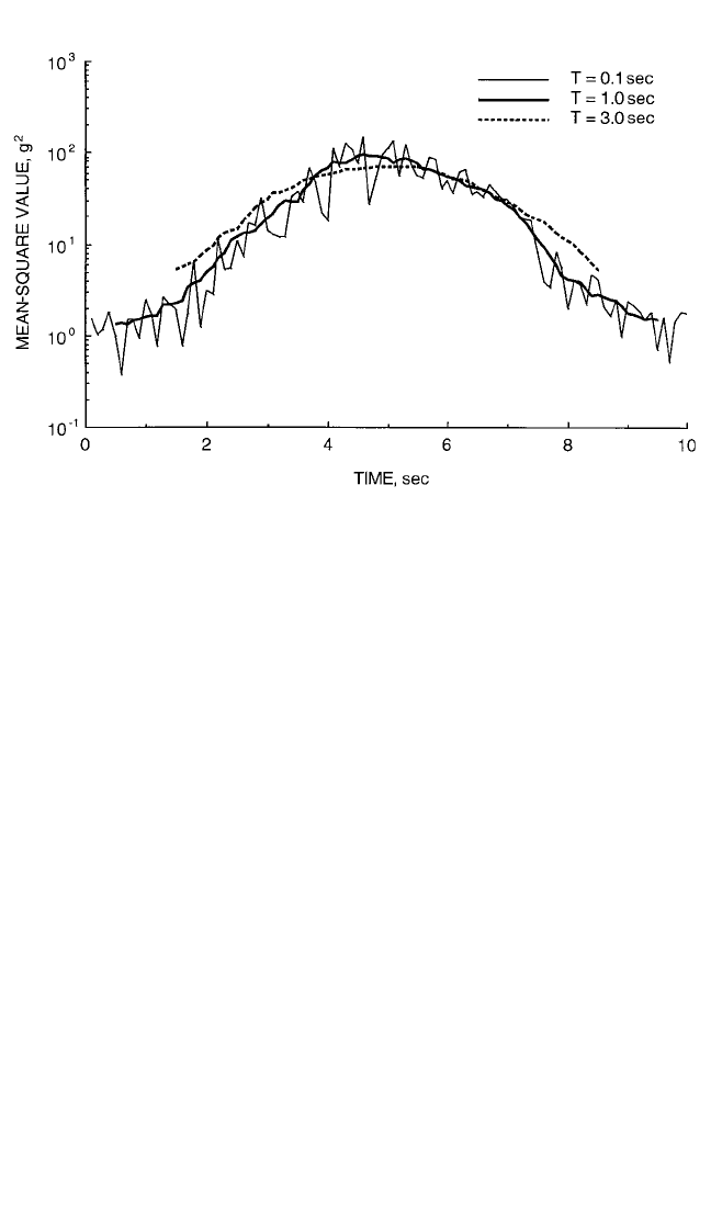
This procedure is illustrated in Fig. 22.9, which shows running average estimates for

the time-varying mean-square value of a nonstationary random vibration record

computed with averaging times of T = 0.1, 1.0, and 3.0 sec. Note that the running

average estimates with T = 0.1 sec reveal substantial random variations from one

estimate to the next, indicative of excessive random estimation errors, while the esti-

mates with T = 3 sec reveal a clear smoothing of the nonstationary trend in the data,

indicative of an excessive time interval bias error. The averaging time of T = 1 sec

provides a good compromise between the suppression of random and bias errors in

the data analysis.

Instantaneous Line Spectrum for Deterministic Data. Again referring to Table

22.5, the most common way to analyze the spectral characteristics of nonstationary

deterministic vibration data is to estimate the instantaneous line spectrum defined in

Eq. (22.19) by a sequence of line spectra computed over the time intervals defined in

Eq. (22.34) or (22.35). The resulting collection of line spectra is commonly referred to

as a waterfall plot or a cascade plot. An illustration of a waterfall plot computed from

a sample record of nonstationary deterministic vibration data is shown in Fig. 14.25.

For a spectral analysis using Fourier transforms, the averaging time T = N∆t and

the frequency resolution ∆f = 1/T = 1/(N∆t) are obviously interrelated. It follows that

there must always be a compromise between these two analysis parameters. On the

22.26 CHAPTER TWENTY-TWO

FIGURE 22.9 Running mean-square value estimates for nonstationary vibration data.

8434_Harris_22_b.qxd 09/20/2001 12:06 PM Page 22.26

one hand, the averaging time must be longer than the period of the lowest instanta-

neous frequency component in the data at any time covered by the sample record.

On the other hand, the frequency resolution must be narrower than the minimum

frequency separation of any two instantaneous frequency components in the data at

any time covered by the sample record. This compromise will generally be achiev-

able for nonstationary deterministic vibration data that would be periodic if they

were stationary. In this case, assuming the maximum period at any time covered by

the sample record is T

, it follows that ∆f < 1/T

if T > T

. However, for almost-

periodic deterministic vibration data, there may be two spectral components that, at

some instant, might be separated by less than ∆f = 1/T where T > T

. See Chap. 14 for

further details on the computation of waterfall plots and other procedures for the

analysis of nonstationary deterministic vibration data.

Instantaneous Power Spectra for Random Data. Referring to Table 22.5, the

instantaneous power spectrum for nonstationary random vibration data requires an

averaging operation to suppress the statistical sampling errors associated with all

random data analysis, as suggested by the expected value operation in Eq. (22.21).

This averaging operation can be accomplished in several ways. For example, the

sample record could be divided into a sequence of contiguous time intervals of

appropriate durations and a power spectrum for the data in each time interval com-

puted using the ensemble-averaging procedure detailed in Table 22.3. However, the

most straightforward way is to compute the instantaneous power spectrum using the

bandpass filtering approach in Fig. 22.5, and computing a running average of the

squared output of each bandpass filter centered at frequency f

with an averaging

time of T

= N

∆t; i = 1,2,3,...,as shown in Table 22.5. For reasons to be discussed

shortly, a fixed averaging time of T = N∆t commonly can be used for all frequency

bands with good results.

A straightforward but time-consuming way to select an appropriate averaging time

for an instantaneous power spectrum estimate with bandpass digital filters is to use the

trial-and-error procedure illustrated for nonstationary mean-square value estimates in

Fig. 22.9, except now the optimum averaging time would have to be determined sepa-

rately for each frequency resolution bandwidth B

. On the other hand, the problem

can also be approached analytically by determining the averaging time and resolution

bandwidth that will minimize the total mean-square error in the estimate, similar to

the procedure given in Eqs. (22.31) through (22.33) for stationary random vibration

data. In this case, however, there is a third error that must be included in the total

mean-square error, namely, a time resolution bias error caused by smoothing through

the time-varying values of the instantaneous power spectrum. A maximum value for

the normalized time resolution bias error can be approximated by

[

(f)] =



(22.36)

where T

is the half-power point duration about the maximum power-spectral den-

sity value in the ith resolution bandwidth, that is, the time interval between the time

before and the time t

after that time t

when the maximum value occurs such that

) = W

)/2. Ideally, this time duration should be determined

individually for each frequency resolution bandwidth, but it will often suffice to use

a single value for T

determined from the estimate for the time-varying mean-

square value of the data, as illustrated in Fig. 22.9.Adding Eq. (22.36) with a constant

value T

to Eq. (22.32), taking partial derivatives with respect to T and B

, equating

to zero, and solving the two simultaneous equations, yields the optimum averaging

time and resolution bandwidth as

2π



CONCEPTS IN VIBRATION DATA ANALYSIS 22.27

8434_Harris_22_b.qxd 09/20/2001 12:06 PM Page 22.27

(f) = 1.31 T

5/6

/(ζf)

1/6

(f) = 1.94(ζf)

5/6

1/6

(22.37)

Note in Eq. (22.37) that the averaging time T

(f) is a function of the −

⁄6 power of the

product ζf, while the resolution bandwidth B

(f) is a function of the

⁄6 power of the

product ζf. Assuming all structural resonances have approximately the same damp-

ing ratio, this means a fixed averaging time and a constant percentage resolution

bandwidth will provide near-optimum results in terms of a minimum mean-square

error in the instantaneous power-spectrum estimate. For example, assume the meas-

ured vibration response of a structure exposed to a nonstationary random excitation

has a time-varying mean-square value similar to that shown in Fig. 22.9, where the

half-power duration is about T

≈ 2.5 sec. Further assume all resonant modes of the

structure have a damping ratio of ζ=0.05. From Eq. (22.37), the optimum averaging

time for the computation of an instantaneous power spectrum of the nonstationary

structural vibration is T

(f) = 4.63f

−1/6

, while the optimum resolution bandwidth is

(f) = 0.137f

5/6

. Hence, if the frequency range of the analysis is, say, 10 Hz to 1000

Hz, the optimum averaging time for the analysis decreases from T

= 3.15 sec at 10

Hz to T

= 1.46 sec at 1000 Hz, while the optimum resolution bandwidth increases

from B

= 0.933 Hz at f = 10 Hz [B

(f) = 0.0933f] to B

= 43.3 Hz at f = 1000 Hz

(f) = 0.0433f]. It follows that an analysis with a fixed averaging time of about T =

2.5 sec and a constant percentage resolution bandwidth of

⁄12 octave, which is equiv-

alent to B

(f) = 0.058f, will provide relative good instantaneous spectral estimates

over the entire frequency range of interest. See Ref. 1 for details on specialized pro-

cedures for analyzing special cases of nonstationary random vibration data.

REFERENCES

1. Bendat, J. S., and A. G. Piersol:“Random Data:Analysis and Measurement Procedures,” 3d

ed., John Wiley & Sons, Inc., New York, 2000.

2. Himelblau, H., et al.: “Handbook for Dynamic Data Acquisition and Analysis,” IEST Rec-

ommended Practice DTE012.1, Institute of Environmental Sciences and Technology,

Mount Prospect, Ill., 1994.

3. Bendat, J. S.: “Nonlinear Systems Techniques and Applications,” John Wiley & Sons, Inc.,

New York, 1998.

4. Wirching, P. H., T. L. Paez, and H. Ortiz: “Random Vibrations, Theory and Practice,” John

Wiley & Sons, Inc., New York, 1995.

5. Nigam, N. C.:“Introduction to Random Vibrations,” MIT Press, Cambridge, Mass., 1983.

6. Newland, D. E.: “Random Vibrations, Spectral Analysis and Wavelet Analysis,” 3d ed.,

Longman, Essex, England, 1993.

7. Bendat, J. S., and A. G. Piersol: “Engineering Applications of Correlation and Spectral

Analysis,” 2d ed., John Wiley & Sons, Inc., New York, 1993.

8. Gardner, W. A.: “Cyclostationarity in Communications and Signal Processing,” IEEE

Press, New York, 1994.

9. Cohen, L.: “Time-Frequency Analysis,” Prentice-Hall, Inc., Upper Saddle River, N.J., 1995.

10. Schmidt, H.: J. Sound and Vibration, 101(3):347 (1985).

22.28 CHAPTER TWENTY-TWO

8434_Harris_22_b.qxd 09/20/2001 12:06 PM Page 22.28

CHAPTER 23

CONCEPTS IN

SHOCK DATA ANALYSIS

Sheldon Rubin

INTRODUCTION

This chapter discusses the interpretation of shock measurements and the reduction

of data to a form adapted to further engineering use. Methods of data reduction also

are discussed.A shock measurement is a trace giving the value of a shock parameter

versus time over the duration of the shock, referred to hereafter as a time-history.

The shock parameter may define a motion (such as displacement, velocity, or accel-

eration) or a load (such as force, pressure, stress, or torque). It is assumed that any

corrections that should be applied to eliminate distortions resulting from the instru-

mentation have been made.The trace may be a pulse or transient. Concepts in vibra-

tion data analysis are discussed in Chap. 22.

Examples of sources of shock to which this discussion applies are earthquakes

(see Chap. 24), free-fall impacts, collisions, explosions, gunfire, projectile impacts,

high-speed fluid entry, aircraft landing and braking loads, and spacecraft launch and

staging loads.

BASIC CONSIDERATIONS

Often, a shock measurement in the form of a time-history of a motion or loading

parameter is not useful directly for engineering purposes. Reduction to a different

form is then necessary, the type of data reduction employed depending upon the

ultimate use of the data.

Comparison of Measured Results with Theoretical Prediction. The correlation

of experimentally determined and theoretically predicted results by comparison of

records of time-histories is difficult. Generally, it is impractical in theoretical analy-

ses to give consideration to all the effects which may influence the experimentally

obtained results. For example, the measured shock often includes the vibrational

response of the structure to which the shock-measuring device is attached. Such

vibration obscures the determination of the shock input for which an applicable the-

ory is being tested; thus, data reduction is useful in minimizing or eliminating the

23.1

8434_Harris_23_b.qxd 09/20/2001 12:02 PM Page 23.1

irrelevancies of the measured data to permit ready comparison of theory with cor-

responding aspects of the experiment. It often is impossible to make such compar-

isons on the basis of original time-histories.

Calculation of Structural Response. In the design of equipment to withstand

shock, the required strength of the equipment is indicated by its response to the

shock. The response may be measured in terms of the deflection of a member of the

equipment relative to another member or by the magnitude of the dynamic loads

imposed upon the equipment. The structural response can be calculated from the

time-history by known means; however, certain techniques of data reduction result

in descriptions of the shock that are related directly to structural response.

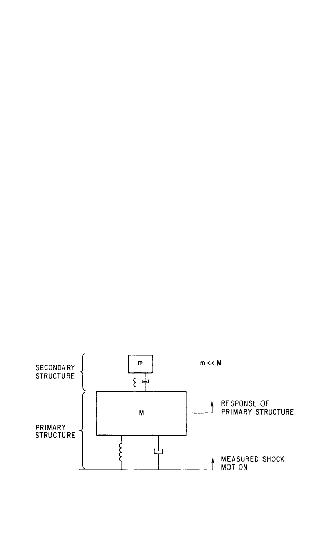
As a design procedure it is convenient to represent the equipment by an appro-

priate model that is better adapted to analysis (see Chap. 41). A typical model is

shown in Fig. 23.1; it consists of a secondary structure supported by a primary

structure. Each structure is represented as a lumped-parameter single degree-of-

freedom system with the secondary mass m much smaller than the primary mass M

so that the response of the primary mass is unaffected by the response of the sec-

ondary mass. The response of the primary mass to an input shock motion is the

input shock motion to the secondary structure. Depending upon the ultimate

objective of the design work, certain characteristics of the response of the model

must be known:

1. If design of the secondary structure is to be effected, it is necessary to know the

time-history of the motion of the primary structure. Such motion constitutes the

excitation for the secondary structure.

2. In the design of the primary structure, it is necessary to know the deflection of

such structure as a result of the shock, either the time-history or the maximum

value.

By selection of suitable data reduction methods, response information useful in

the design of the equipment is obtained from the original time-history.

23.2 CHAPTER TWENTY-THREE

FIGURE 23.1 Commonly used structural model consisting of a primary and a

secondary structure.

Laboratory Simulation of Measured Shock. Because of the difficulty of using

analytical methods in the design of equipment to withstand shock, it is common

practice to prove the design of equipments by laboratory tests that simulate the

anticipated actual shock conditions. Unless the shock can be defined by one of a

8434_Harris_23_b.qxd 09/20/2001 12:02 PM Page 23.2

few simple functions, it is not feasible to reproduce in the laboratory the complete

time-history of the actual shock experienced in service. Instead, the objective is to

synthesize a shock having the characteristics and severity considered significant in

causing damage to equipment. Then, the data reduction method is selected so that

it extracts from the original time-history the parameters that are useful in specify-

ing an appropriate laboratory shock test. Shock testing machines are discussed in

Chap. 26.

EXAMPLES OF SHOCK MOTIONS

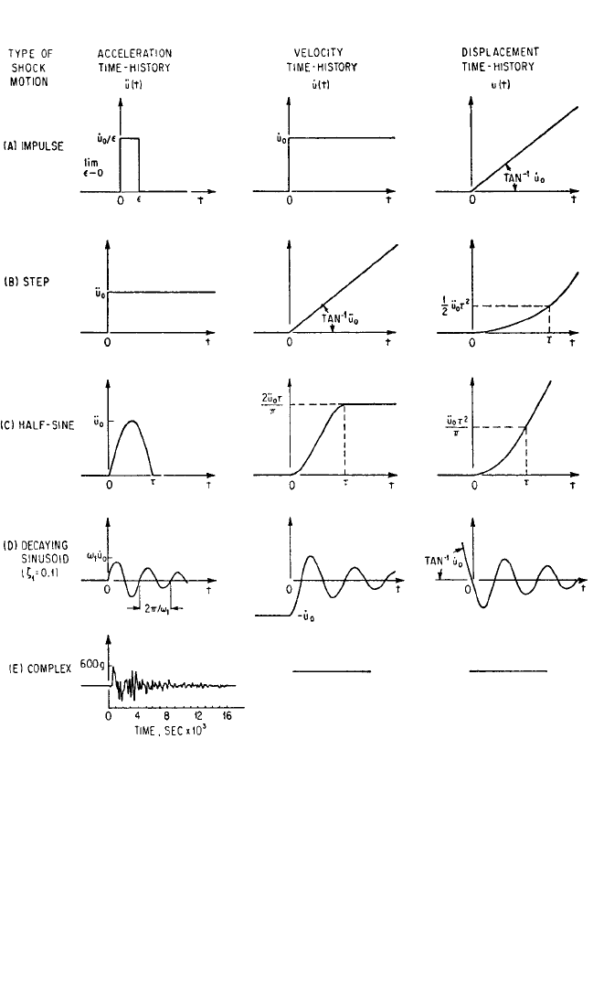
Five examples of shock motions are illustrated in Fig. 23.2 to show typical character-

istics and to aid in the comparison of the various techniques of data reduction. The

acceleration impulse and the acceleration step are the classical limiting cases of

shock motions. The half-sine pulse of acceleration, the decaying sinusoidal accelera-

tion, and the complex oscillatory-type motion typify shock motions encountered fre-

quently in practice.

In selecting data reduction methods to be used in a particular circumstance, the

applicable physical conditions must be considered. The original record, usually a

time-history, may indicate any of several physical parameters; e.g., acceleration,

force, velocity, or pressure. Data reduction methods discussed in subsequent sections

of this chapter are applicable to a time-history of any parameter. For purposes of

illustration in the following examples, the primary time-history is that of accelera-

tion; time-histories of velocity and displacement are derived therefrom by integra-

tion. These examples are included to show characteristic features of typical shock

motions and to demonstrate data reduction methods.

ACCELERATION IMPULSE OR STEP VELOCITY

The delta function d(t) is defined mathematically as a function consisting of an infi-

nite ordinate (acceleration) occurring in a vanishingly small interval of abscissa

(time) at time t = 0 such that the area under the curve is unity. An acceleration time-

history of this form is shown diagrammatically in Fig. 23.2A. If the velocity and dis-

placement are zero at time t = 0, the corresponding velocity time-history is the

velocity step and the corresponding displacement time-history is a line of constant

slope, as shown in the figure. The mathematical expressions describing these time

histories are

ü(t) = ˙u

d(t) (23.1)

where d(t) = 0 when t ≠ 0, d(t) =∞when t = 0, and



∞

−∞

d(t) dt = 1. The acceleration can

be expressed alternatively as

ü(t) = lim

 → 0

˙u

/ [0 < t < ] (23.2)

where ü(t) = 0 when t < 0 and t > . The corresponding expressions for velocity and

displacement for the initial conditions u = ˙u = 0 when t < 0 are

˙u(t) = ˙u

[t > 0] (23.3)

u(t) = ˙u

t [t > 0] (23.4)

CONCEPTS IN SHOCK DATA ANALYSIS 23.3

8434_Harris_23_b.qxd 09/20/2001 12:02 PM Page 23.3

ACCELERATION STEP

The unit step function 1(t) is defined mathematically as a function which has a value

of zero at time less than zero (t < 0) and a value of unity at time greater than zero

(t > 0). The mathematical expression describing the acceleration step is

ü(t) = ü

1(t) (23.5)

23.4 CHAPTER TWENTY-THREE

FIGURE 23.2 Five examples of shock motions.

8434_Harris_23_b.qxd 09/20/2001 12:02 PM Page 23.4

where 1(t) = 1 for t > 0 and 1(t) = 0 for t < 0. An acceleration time-history of the unit

step function is shown in Fig. 23.2B; the corresponding velocity and displacement

time-histories are also shown for the initial conditions u = ˙u = 0 when t = 0.

˙u(t) = ü

t [t > 0] (23.6)

u(t) =

⁄2ü

[t > 0] (23.7)

The unit step function is the time integral of the delta function:

1(t) =



−∞

d(t) dt [t > 0] (23.8)

HALF-SINE ACCELERATION

A half-sine pulse of acceleration of duration τ is shown in Fig. 23.2C; the correspon-

ding velocity and displacement time-histories also are shown, for the initial condi-

tions u = ˙u = 0 when t = 0. The applicable mathematical expressions are

ü(t) = ü

sin



[0 < t <τ]

ü(t) = 0 when t < 0 and t >τ

(23.9)

˙u(t) =



1 − cos



[0 < t <τ]

˙u(t) = [t >τ]

(23.10)

u(t) =



− sin



[0 < t <τ]

u(t) =



− 1



[t >τ]

(23.11)

This example is typical of a class of shock motions in the form of acceleration pulses

not having infinite slopes.

DECAYING SINUSOIDAL ACCELERATION

A decaying sinusoidal trace of acceleration is shown in Fig. 23.2D; the corresponding

time-histories of velocity and displacement also are shown for the initial conditions

u˙ =−˙u

and u = 0 when t = 0. The applicable mathematical expression is

ü(t) = e

−ζ

sin (1



−



t + sin

−1

(2ζ

1



−



)) [t > 0] (23.12)

where ω

is the frequency of the vibration and ζ

is the fraction of critical damping

corresponding to the decrement of the decay. Corresponding expressions for veloc-

ity and displacement are

˙u



1



−





πt



πt



2ü



πt



πt



CONCEPTS IN SHOCK DATA ANALYSIS 23.5

8434_Harris_23_b.qxd 09/20/2001 12:02 PM Page 23.5

˙u(t) = e

−ζ

cos (1



−



t + sin

−1

)[t > 0] (23.13)

where ˙u(t) =−˙u

when t < 0.

u(t) =− e

−ζ

sin (1



−



t)[t > 0] (23.14)

where u(t) =−˙u

t when t < 0.

COMPLEX SHOCK MOTION

The trace shown in Fig. 23.2E is an acceleration time-history representing typical

field data. It cannot be defined by an analytic function. Consequently, the corre-

sponding velocity and displacement time-histories can be obtained only by numeri-

cal, graphical, or analog integration of the acceleration time-history.

CONCEPTS OF DATA REDUCTION

Consideration of the engineering uses of shock measurements indicates two basically

different methods for describing a shock: (1) a description of the shock in terms of its

inherent properties, in the time domain or in the frequency domain; and (2) a descrip-

tion of the shock in terms of the effect on structures when the shock acts as the exci-

tation. The latter is designated reduction to the response domain. The following

sections discuss concepts of data reduction to the frequency and response domains.

Whenever practical, the original time-history should be retained even though the

information included therein is reduced to another form. The purpose of data reduc-

tion is to make the data more useful for some particular application. The reduced

data usually have a more limited range of applicability than the original time-history.

These limitations must be borne in mind if the data are to be applied intelligently.

DATA REDUCTION TO THE FREQUENCY DOMAIN

Any nonperiodic function can be represented as the superposition of sinusoidal

components, each with its characteristic amplitude and phase.

This superposition is

the Fourier spectrum, as defined in Eq. (23.55). It is analogous to the Fourier com-

ponents of a periodic function (Chap. 22). The Fourier components of a periodic

function occur at discrete frequencies, and the composite function is obtained by

superposition of components. By contrast, the classical Fourier spectrum for a non-

periodic function is a continuous function of frequency, and the composite function

is achieved by integration. The following sections discuss the application of the con-

tinuous Fourier spectrum to describe the shock motions illustrated in Fig. 23.2. A dis-

crete realization of the Fourier spectrum is given by Eq. (22.26).

Acceleration Impulse. Using the definition of the acceleration pulse given by Eq.

(23.2) and substituting this for f(t) in Eq. (23.55),

F(ω) = lim

 → 0



−jωt

dt (23.15)

˙u





˙u



1



−



˙u



1



−



23.6 CHAPTER TWENTY-THREE

8434_Harris_23_b.qxd 09/20/2001 12:02 PM Page 23.6