Hassani S. Mathematical Methods: For Students of Physics and Related Fields

Подождите немного. Документ загружается.

556 First-Order Diﬀerential Equations

23.3 First-Order Linear Diﬀerential Equations

A linear DE is a sum of terms each of which is the product of a derivative

of the dependent variable (say y) and a function of the independent variable

(say x). The highest order of the derivative is called the order of the linear

order of a linear

DE. The most general ﬁrst-order linear diﬀerential equation (FOLDE) is

(x)y



+ p

(x)y = q(x) ⇔ p

dy +(p

y − q) dx =0. (23.9)

If this equation is to have a solution, then by the argument at the end of the

last subsection, it must have at least one integrating factor. Let μ(x, y)bean

integrating factor. Then there exists v(x, y) such that

dv = μ(p

y − q) dx + μp

dy =0

The necessary and suﬃcient condition for this to hold is

∂

∂y

[μ(p

y − q)] =

∂

∂x

(μp

To simplify the problem, let us assume that μ is a function of x only (we are

looking for any integrating factor, not the most general one). Then the above

condition leads to the diﬀerential equation

μp

(μp

)=p

dμ

+ μ

(23.10)

dμ

= μ



−



⇒

dμ

dx −

Integrating both sides gives

ln μ =

dx −ln p

+lnC ⇒ ln



μp



μp

= e



dx/p

⇒ μ =



dx/p

Neglecting the unimportant constant of integration, we have found the in-

tegrating factor μ =exp[(



dx/p

)]/p

. Now multiply both sides of the

original equation by μ to obtain

μp



+ μp

y = μq. (23.11)

With the identity μp



≡ (μp



− (μp

)



y and the fact that (μp

)



= μp

[the ﬁrst equality of Equation (23.10)], Equation (23.11) becomes

(μp

y)=μq ⇒ μp

y =

μ(x)q(x) dx + C.

23.3 First-Order Linear Diﬀerential Equations 557

Therefore, explicit solution of

a general

ﬁrst-order linear

diﬀerential

equation

Theorem 23.3.1. Any FOLDE of the form p

(x)y



(x)y = q(x),inwhich

, p

,andq are continuous functions in some interval (a, b), has a general

solution

y = f(x)=

μ(x)p

(x)



C +

μ(x)q(x) dx



, (23.12)

where C is an arbitrary constant, and

μ(x)=

(x)

exp



(x)



. (23.13)

Example 23.3.2.

In an electric circuit with a resistance R and a capacitance C, detailed treatment

of an RC circuitKirchhoﬀ’s law gives rise to the equation RdQ/dt+ Q/C = V (t), where V (t)isthe

time-dependent voltage and Q is the (instantaneous) charge on the capacitor. This

is a simple FOLDE with p

= R, p

=1/C,andq = V . The integrating factor is

μ(t)=

exp





t/RC

which yields

Q(t)=

μ(t)p

(t)



B +

t/RC

V (t) dt



= Be

−t/RC

t/RC

V (t) dt.

Recall that an indeﬁnite integral can be written as a deﬁnite integral whose upper

limit is the independent variable—in which case we need to use a diﬀerent symbol

for the integration variable. For the arbitrary lower limit, choose zero. We then

have

Q(t)=Be

−t/RC

s/RC

V (s) ds. (23.14)

Let Q(0) ≡ Q

be the initial charge. Then, substituting t = 0 in (23.14), we get

= B and the charge at time t will be given by

Q(t)=Q

−t/RC

s/RC

V (s) ds. (23.15)

As a speciﬁc example, assume that the voltage is a constant V

,asinthecase

of a battery. Then the charge on the capacitor as a function of time will be

Q(t)=Q

−t/RC

+ V

C(1 − e

−t/RC

It is interesting to note that the ﬁnal charge Q(∞)isV

C, independent of the initial

charge. Intuitively, this is what we expect, of course, as the “capacity” of a capacitor

to hold electric charge should not depend on its initial charge.



558 First-Order Diﬀerential Equations

Example 23.3.3. As a concrete illustration of the general formula derived in the

previous example, we ﬁnd the charge on a capacitor in an RC circuit when a voltage,

V (t)=V

cos ωt, is applied to it for a period T andthenremoved. V (t)canthus

be written as

V (t)=

cos ωt if t<T,

0ift>T.

The general solution is given as Equation (23.15). We have to distinguish between

two regions in time, t<T and t>T.

(a) For t<T, we have (using a table of integrals)

Q(t)=Q

−t/RC

s/RC

cos ωsds

= Q

−t/RC

(1/RC)

+ ω



−

−t/RC

cos ωt

+ ω sin ωt



If T  RC, and we wait long enough,

i.e., t  RC, then only the oscillatory part

survives due to the large negative exponents of the exponentials. Thus,

Q(t) ≈

(1/RC)

+ ω



cos ωt

+ ω sin ωt



The charge Q(t) oscillates with the same frequency as the driving voltage.

(b) For t>T, the integral goes up to T beyond which V (t) is zero. Hence, we have

Q(t)=Q

−t/RC

s/RC

cos ωsds

= Q

−t/RC

(1/RC)

+ ω



−

−t/RC

+ e

(T −t)/RC



cos ωT

+ ω sin ωT



We note that the oscillation has stopped (sine and cosine terms are merely constants

now), and for t −T  RC, the charge on the capacitor becomes negligibly small: If

there is no applied voltage, the capacitor will discharge.



Although ﬁrst-order linear DEs can always be solved—yielding solutions as

given in Equation (23.12)—no general rule can be applied to solve a general

FODE. Nevertheless, it can be shown that a solution of such a DE always

exist, and, under some mild conditions, this solution is unique. Some special

nonlinear FODEs can be solved using certain techniques some of which are

described in the following examples as well as the problems at the end of the

chapter.

Example 23.3.4.

In Problem 23.11 you are asked to ﬁnd the velocity of a fallingfalling object with

air resistance object when the air drag is proportional to velocity. This is a good approximation

at low velocities for small objects; at higher speeds, and for larger objects, the drag

force becomes proportional to higher powers of speed. Let us consider the case when

the drag force is proportional to v

. Then the second law of motion becomes

= mg − bv

⇒

= g − γv

,γ≡

Of course, we still assume that t<T.

23.3 First-Order Linear Diﬀerential Equations 559

This equation can be written as

g −γv

= dt ⇒

− v

= γdt, A

. (23.16)

Now we rewrite

− v



v + A

−

v − A



multiply both sides of Equation (23.16) by 2A and integrate to obtain

ln |v + A|−ln |v − A| =2Aγt +lnC,

where we have written the constant of integration as ln C for convenience. This

equation can be rewritten as



v + A

v − A



= Ce

2Aγt

Suppose that at t = 0, the velocity of the falling object is v

,then



+ A

− A



= C

and



v + A

v −A



+ A

− A



2Aγt

Now note that A>0, and v>0 (if we take “down” to be the positive direction).

Therefore, the last equation becomes

v + A

|v −A|

+ A

− A|

2Aγt

Suppose that v

>A; then we can remove the absolute value sign from the RHS,

and since the two sides must agree at t = 0, we can remove the absolute value sign

on the LHS as well. Similarly, if v

<A,thenv<Aas well. It follows that

v + A

v − A

+ A

− A

2Aγt

⇒ (v + A)(v

− A)=(v − A)(v

+ A)e

2Aγt

Solving for v gives

v = A

+ A)e

2Aγt

+ v

− A

+ A)e

2Aγt

− (v

− A)

= A

2Aγt

+1)+A(e

2Aγt

− 1)

2Aγt

− 1) + A(e

2Aγt

+1)

(23.17)

= A

cosh(Aγt)+A sinh(Aγt)

sinh(Aγt)+A cosh(Aγt)

It follows from Equation (23.17) that at t = 0, the velocity is v

,asweexpect. It

also shows that, when t →∞, the velocity approaches A =



g/γ, the so-called

terminal velocity. This is the velocity at which the gravitational force and the terminal velocity

drag force become equal, causing the acceleration of the object to be zero. The

terminal velocity can thus be obtained directly from the second law without solving

the diﬀerential equation.

560 First-Order Diﬀerential Equations

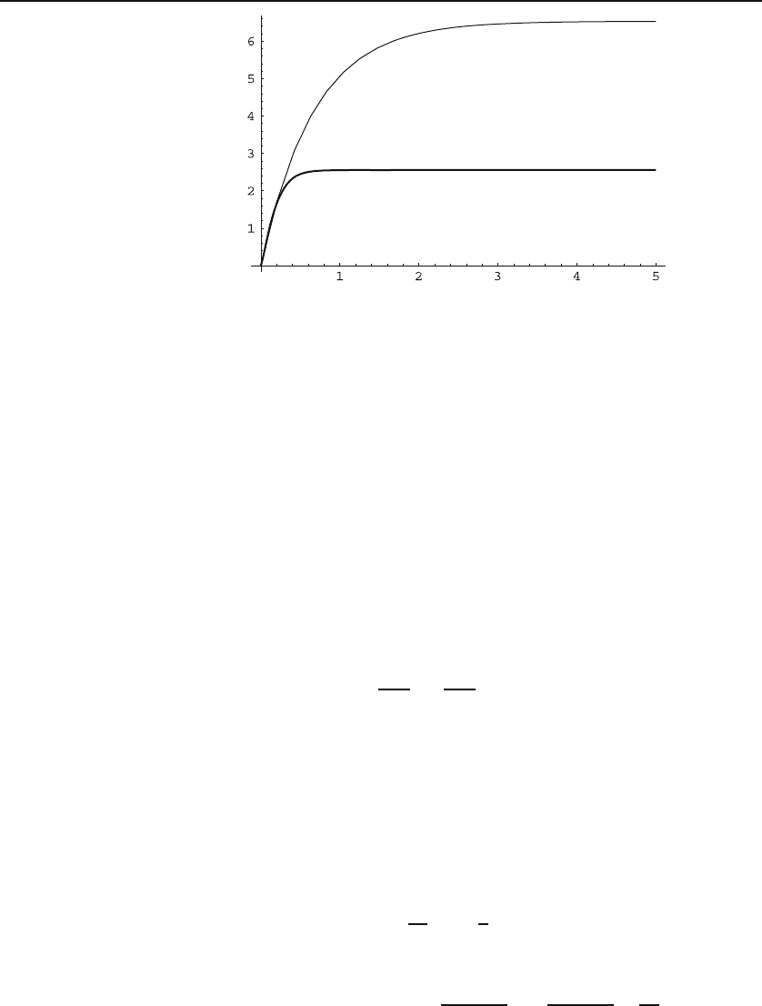
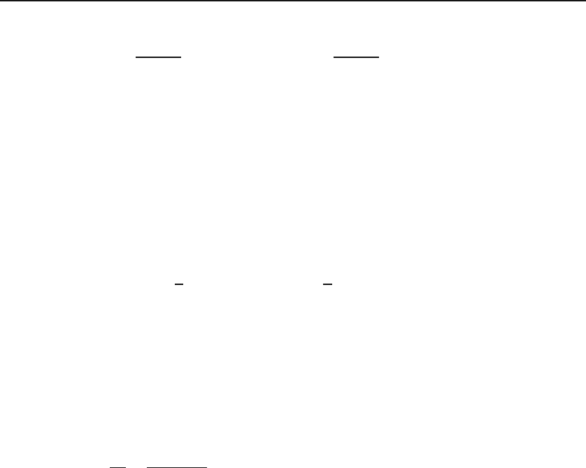
Figure 23.1: The achievement of terminal velocity for a drag force that is proportional

to the square of speed (the heavy curve) is considerably faster than for a drag force that

is linear in speed (the light curve) if γ has the same numerical value for both cases.

Figure 23.1 shows the plot of speed as a function of time for the two cases of the

drag force being proportional to v and v

with the same proportionality constant.

Because of the higher power of speed, the terminal velocity is achieved considerably

more quickly for v

force than for v force. Furthermore, as the ﬁgure shows clearly,

the terminal speed itself is much smaller in the former case. Since larger surfaces

provide a v

drag force, parachutes that have very large surface are desirable.



Example 23.3.5. We consider here some other examples of (nonlinear) FODEs

whose solutions are available:

(a) Bernoulli’s FODE: This equation is of the form y



+ p(x)y + q(x)y

=0whereBernoulli’s FODE

n = 1. This DE can be simpliﬁed if we substitute y = u

and choose r appropriately.

In terms of u, the DE becomes



p(x)

u +

q(x)

nr−r+1

=0.

The simplest DE—whose solution could be found by a simple integration—would

be obtained if the exponent of the last term could be set equal to 1. But this would

require r to be zero, which is not acceptable. The next simplest DE results if we set

the exponent equal to zero, i.e., if r =1/(1 − n). Then the DE becomes



+(1− n)p(x)u +(1− n)q(x)=0

which is a ﬁrst-order linear DE whose solution we have already found.

(b) Homogeneous FODE:ThisDEisoftheformhomogeneous

FODE

= w





To ﬁnd the solution, make the obvious substitution u = y/x,toobtainy



= u + xu



and

u + xu



= w(u) ⇒ u



w(u) −u

⇒

w(u) −u

23.4 Problems 561

with the solution

ln x =

w(t) − t

or x =exp

y/x

w(t) − t

where c is an arbitrary constant to be determined by the initial conditions.



23.4 Problems

23.1. Suppose that region D is contractible to zero. Using the equivalence of

the vanishing of curl and vanishing of closed line integrals, show that ∂M/∂y =

∂N/∂x is both necessary and suﬃcient condition for Mdx+Ndyto be exact.

23.2. Verify that μ = C/(x

) is an integrating factor of xdy−ydxwhich

gives rise to

v =tan

−1





= constant ⇒

= C



for a solution of xdy− ydx.

23.3. Find the general solution of Bernoulli’s FODE



+ p(x)y + q(x)y

=0 where n =1.

Hint: See Example 23.3.5.

23.4. Find a solution to the linear fractional DE

x + a

x + b

where a

= a

Hint: Divide the numerator and denominator by x to obtain a homogeneous

FODE.

23.5. Lagrange’s FODE is y − xp(y



) − q(y



)=0. Lagrange’s FODE

(a) Let y



= t and consider x as a function of t. Using the chain rule, ﬁnd

dx/dt in terms of dy/dt.

(b) Diﬀerentiate Lagrange’s DE with respect to t. Use the result of this

diﬀerentiation and that of (a) to arrive at [t −p(t)] ˙x − ˙px =˙q,wherethedot

indicates diﬀerentiation with respect to t.

t = p(t)andt = p(t).

23.6. Let u(x, y)=C be a solution of the DE Mdx+ Ndy= 0. Show that:

(a) (∂u/∂x)/M =(∂u/∂y)/N ;and

(b) μ(x, y) ≡ (∂u/∂x)/M is an integrating factor for the DE.

23.7. Use direct diﬀerentiation to show that the function given in Equation

(23.12) solves the FOLDE of Equation (23.9).

562 First-Order Diﬀerential Equations

23.8. Analyze the capacitor’s charge in an RC circuit in which a constant

potential V

is applied for a time T>0 and then disconnected. Consider the

cases where t<T and t>T.

23.9. Find all functions f (x) whose deﬁnite integral from 0 to x equals the

square of their reciprocal.

23.10. (a) Let p



u = 0 be a homogeneous FOLDE in u.Solveit.(Note

that it can easily be integrated.)

(b) Consider p



+ p

y = q.Lety = uv,whereu is as in (a), and obtain

an equation for v. Solve this equation, and obtain a general solution for



+ p

y = q. This is the method of variation of parameters,whichcan

also be used for second-order diﬀerential equations.

23.11. A falling body in air has a motion approximately described by the DE

mdv/dt = mg − bv,wherev = dx/dt is the velocity of the body. Find this

velocity as a function of time assuming that the object starts from rest.

23.12. Suppose that both the linear (av) and the quadratic (bv

)termsare

present in the fall of an object with air drag.

(a) Solve the DE and ﬁnd the most general solution for the velocity as a

function of time. Hint: Make the substitution u = v + a/2b.

(b) From this general solution, extract the solutions to the cases where only

the linear and only the quadratic terms are present by taking the limits b → 0

and a → 0.

23.13. Take the limit of Equation (23.17) as t →∞and show that it is equal



g/γ.

Chapter 24

Second-Order Linear

Diﬀerential Equations

The majority of problems encountered in physics lead to second order linear

diﬀerential equations (SOLDEs) when the so-called nonlinear terms are ap-

proximated out. Thus, a general treatment of the properties and methods

of obtaining solutions to SOLDEs is essential. In this section, we investigate

their general properties, and leave methods of obtaining their solutions for

the next section and later chapters.

The most general SOLDE is

(x)

+ p

(x)

+ p

(x)y = p

(x). (24.1)

Dividing by p

(x), and writing p for p

, q for p

,andr for p

reduces Equation (24.1) to the normal form,

normal form of a

SOLDE

+ p(x)

+ q(x)y = r(x). (24.2)

Equation (24.2) is equivalent to (24.1) if p

(x) = 0. The points at which p

(x)

vanishes are called the singular points of the DE.

diﬀerence between

singular points of

linear and

nonlinear

diﬀerential

equations

There is a crucial diﬀerence between the singular points of linear DEs and

those of nonlinear DEs. For a nonlinear DE such as (x

− y)y



= x

+ y

the curve y = x

is the collection of singular points. This makes it impossible

to construct solutions y = f (x) that are deﬁned on an interval I =[a, b]of

the x-axis because for any a<x<b,thereisay = x

for which the DE is

undeﬁned. On the other hand, linear DEs do not have this problem because

the coeﬃcients of the derivatives are functions of x only. Therefore, all the

singular “curves” are vertical, and we can ﬁnd intervals on the x-axis in which

the DE is well behaved.

564 Second-Order Linear Diﬀerential Equations

24.1 Linearity, Superposition, and Uniqueness

The FOLDE has only one solution; and we found this solution in closed form

in Equation (23.12). The SOLDE may have (in fact, it does) more than one

solution. Therefore, it is important to know how many solutions to expect for

a SOLDE and what relation (if any) exists between these solutions.

We write Equation (24.1) as

L[y]=p

where L ≡ p

+ p

. (24.3)

It is clear that L is a linear operator

bywhichwemeanthatforconstants

α and β, L[αy

+ βy

]=αL[y

]+βL[y

]. In particular, if y

and y

are two

solutions of Equation (24.3), then

L[y

− y

]=L[y

] −L[y

]=p

− p

=0.

That is, the diﬀerence between any two solutions of a SOLDE is a solution

of the homogeneous equation obtained by setting p

= 0. An immediatehomogeneous

SOLDE

consequence of the linearity of L is that any linear combination of solutions

of the homogeneous SOLDE (HSOLDE) is also a solution. This is called the

superposition principle.

superposition

principle

We saw in the introduction to Chapter 22 that, based on physical intu-

ition, we expect to be able to predict the behavior of a physical system if we

know the DE obeyed by that system and equally importantly, the initial data.

Physical intuition also tells us that if the initial conditions are changed by an

inﬁnitesimal amount, then the solutions will be changed inﬁnitesimally. Thus,

the solutions of linear DEs are said to be continuous functions of the initial

conditions. Nonlinear DEs can have completely diﬀerent solutions for two

initial conditions that are inﬁnitesimally close. Since initial conditions cannot

be speciﬁed with mathematical precision in practice, nonlinear DEs lead to

unpredictable solutions, or chaos. This subject has received much attention

in recent years, and we shall present a brief discussion of chaos in Chapter 31.

By its very nature, a prediction is expected to be unique. This expectation

for linear equations becomes—in the language of mathematics—an existence

and a uniqueness theorem. First, we need the following

Theorem 24.1.1. The only solution g(x) of the homogeneous equation y





+ qy =0, deﬁned on the interval [a, b], which satisﬁes g(a)=0=g



(a),is

the trivial solution, g =0.

Let f

and f

be two solutions of (24.2) satisfying the same initial condi-

tions on the interval [a, b]. This means that f

(a)=f

(a)=c and f



(a)=

Recall from Chapter 7 that an operator is a correspondence on a vector space that

takes one vector and gives another. A linear operator is an operator that satisﬁes Equation

(7.3). The vector space on which L acts is the vector space of diﬀerentiable functions.

This conclusion is not limited to the SOLDE; it holds for all linear DEs.

For a proof, see Hassani, S. Mathematical Physics: A Modern Introduction to Its Foun-

dations, Springer-Verlag, 1999, p. 354.

24.1 Linearity, Superposition, and Uniqueness 565



(a)=c



for some given constants c and c



. Then it is readily seen that their

diﬀerence, g ≡ f

− f

, satisﬁes the homogeneous equation [with r(x)=0].

The initial condition that g(x) satisﬁes is clearly g(a)=0=g



(a). By Theo-

rem 24.1.1, g =0orf

= f

. We have just shown uniqueness of

solutions to

SOLDE

Theorem 24.1.2. (Uniqueness Theorem).Ifp and q are continuous on

[a, b], then at most one solution of Equation (24.2) can satisfy a given set of

initial conditions.

The uniqueness theorem can be applied to any homogeneous SOLDE to

ﬁnd the latter’s most general solution. In particular, let f

(x)andf

(x)be

any two solutions of



+ p(x)y



+ q(x)y = 0 (24.4)

deﬁned on the interval [a, b]. Assume that the two vectors v

=(f

(a),f



(a))

and v

=(f

(a),f



(a)) are linearly independent.

Let g(x)beanotherso-

lution. The vector (g(a),g



(a)) can be written as a linear combination of v

and v

, giving the two equations

g(a)=c

(a)+c

(a),



(a)=c



(a)+c



(a).

The function u(x) ≡ g(x) − c

(x) − c

(x) satisﬁes the DE (24.4) and

the initial conditions u(a)=u



(a) = 0. It follows from Theorem 24.1.1 that

u(x)=0org(x)=c

(x)+c

(x). We have proved basis of solutions

Theorem 24.1.3. Let f

and f

be two solutions of the HSOLDE



+ py



+ qy =0,

where p and q are continuous functions deﬁned on the interval [a, b].If

(a),f



(a)) and (f

(a),f



(a)) are linearly independent vectors, then every

solution g(x) of this HSOLDE is equal to some linear combination

g(x)=c

(x)+c

(x),

with constant coeﬃcients c

and c

. The functions f

and f

are called a

basis of solutions of the HSOLDE.

The uniqueness theorem states that only one solution can exist for a

there is also an

existence theorem!

SOLDE which satisﬁes a given set of initial conditions. Whether such a

solution does exist is beyond the scope of the theorem. Under some mild

assumptions, however, it can be shown that a solution does indeed exist. We

shall not prove this existence theorem for a general SOLDE, but shall examine

various techniques of obtaining solutions for speciﬁc SOLDEs in this and the

next two chapters.

If they are not, then one must choose a diﬀerent initial point for the interval.