Health and Safety Executive. Guidelines for use of statistics for analysis of sample inspection of corrosion

Подождите немного. Документ загружается.

5.1

4.9

5.1

4.9

5.2

5.0

4.8

4.7

4.9

5.0

5.1

5.0

4.9

5.1

5.3

5.0

4.8

5.2

Figure 2

Example Readings from Pressure Vessel/Pipe

When ordered the data becomes:

4.7, 4.8, 4.8, 4.9, 4.9, 4.9, 4.9, 5, 5, 5, 5, 5, 5, 5.1, 5.1, 5.1, 5.1, 5.2, 5.2, 5.3

The values are grouped in intervals as tabulated below:

Wall Thickness Frequency

4.7 1

4.8 2

4.9 4

5 6

5.1 4

5.2 2

5.3 1

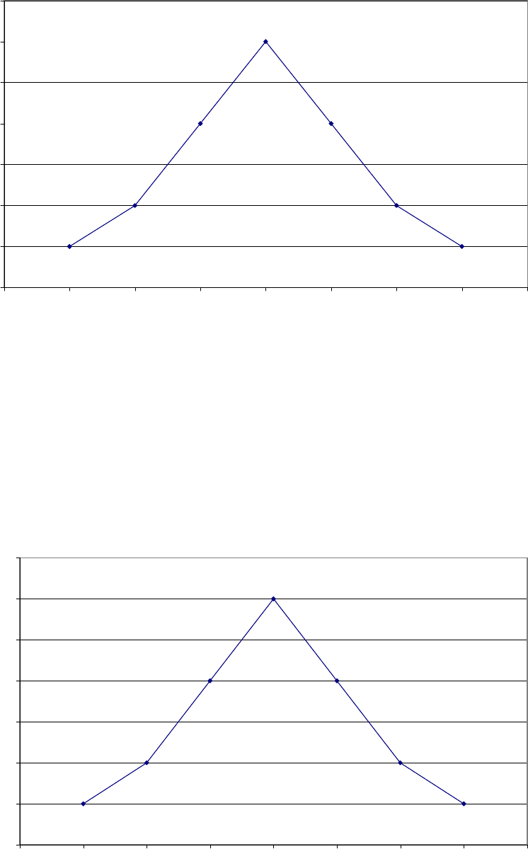
The frequency distribution is a plot of the data in this table as Figure 3.

No of readings

4.6 4.7 4.8 4.9 5 5.1 5.2 5.3

Wall Thickness

Figure 3

Frequency Distribution

This frequency distribution appears to be symmetrical and the central tendency is 5.0.

In order to make use of this pattern in the data it is necessary to convert it into a mathematical

form. The mathematical form must describe the data in Figure 3 or must be a close fit.

Usually one step in this process is to normalise the data by dividing the frequency by the total

number of readings (Figure 4). This is called a normalised frequency distribution (frequency

being the number of readings). Basically the process of fitting the data is one of trial and

error, although tools are available to assist in this process as described below.

0.05

0.1

0.15

0.2

0.25

0.3

0.35

No of readings/total readings

4.6 4.7 4.8 4.9 5 5.1 5.2 5.3

Wall Thickness (mm)

Figure 4

Normalised Frequency Distribution

5.4

No of readings/total readings

0.35

0.3

0.25

0.2

0.15

0.1

0.05

4.6 4.7 4.8 4.9 5 5.1 5.2 5.3

Wall Thickness (mm)

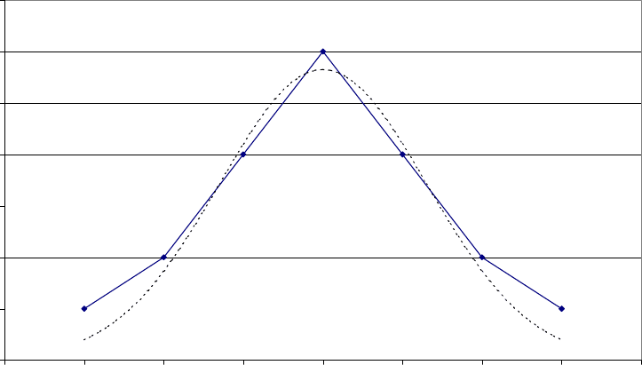
Figure 5

Fitting a Curve (in this case a normal distribution)

There are a number of standard forms of frequency distribution. These have mathematical

equations to describe them, but for the purposes of this document only the general shapes and

the graphical display will be considered. A frequency distribution also has associated with it a

cumulative distribution, which is the sum of the number of readings up to a certain point and

is equivalent to the area under the frequency distribution curve.

Figure 5 shows a normal distribution with a mean of 5.0 and standard deviation of 0.13

adjusted to fit the same scale as the previous frequency distribution. If we believe that this fit

is good enough it is possible to make calculations on the data, for example to estimate the

proportion of the vessel with a wall thickness less than 4.7mm. This is calculated from the

area of the frequency distribution below 4.7mm. This is more easily calculated from the value

of the cumulative distribution at this point. The cumulative distribution is plotted by

successively adding in the number of points/total number. It always reaches a maximum of 1,

for the largest measurement in the data set.

5.4

1.2

Number of Readings up to thickness/Total Numbe

of Readings

0.8

0.6

0.4

0.2

4.6 4.7 4.8 4.9 5 5.1 5.2 5.3

Thickness Reading (mm)

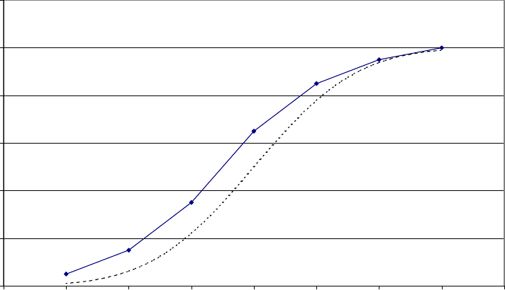
Figure 6

Cumulative Distribution of data and normal distribution curve

The proportion of the wall thickness less than 4.7mm (for example) can be read directly from

this graph.

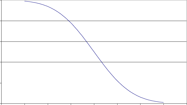
A function derived from the cumulative distribution that will be used in later analyses is

called the survivor function. This is simply the cumulative distribution subtracted from 1.

Figure 7 shows the survivor function for the above normal distribution.

5.4

Proportion of readings greater than given thicknes

0.8

0.6

0.4

0.2

4.6 4.7 4.8 4.9 5 5.1 5.2 5.3

Wall Thickness (mm)

Figure 7

Survivor Function for Normal Distribution

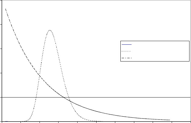
The choice of distribution for the calculations is crucial. Each distribution has a different

shape and the wrong choice can lead to erroneous conclusions. For example two shapes which

may represent certain corrosion types are the lognormal and exponential distributions. The

basic shapes of the frequency distributions for these are given in Figure 8. It is also important

to note that the accuracy of the parameters of the distribution, and the confidence limits

eventually produced, depend on the number of data points used.

When an entire population of a defect is available, for example given a detailed (100%)

surface scan covering an entire vessel, then statistical analyses of the data generally produce a

fundamental or underlying distribution pattern. In this case all data values are fully defined.

Typical fundamental distribution patterns include those shown in Figure 8, but could also

include Poisson or Gaussian distributions.

In practice complete data population sets rarely occur. For example 100% scanning of a

vessel would be considered impractical. Accordingly statistical treatments and procedures

have arisen over the years to allow predictions to be made on the basis of limited sample

information, where the sample is used to infer the greater population behaviour. N.B. A

statistical sample which contains less than an entire population of data may follow the

distribution of its parent population and this may be a fundamental distribution.

5.4

0.5

1.5

2.5

0 0.5 1 1.5 2 2.5 3 3.5 4 4.5 5

Frequency

Normal Distribution

Lognormal distribution

Exponential Distribution

Value of Distribution

Figure 8

Different Distribution Shapes

One special example that is important in the context of inspection is the family of extreme

value distributions. Instead of being constructed from all the readings taken, they are

constructed from the extreme values of groups of the data. Usually for inspection the data

will be grouped in areas. So for example if the results from Figure 2 are in circumferential

bands, the lower extreme values will be 4.9, 4.8, 4.7, 4.9, 4.8 and these will form a

distribution of their own called an extreme value distribution.

4.1.1 Extreme Value Distribution

The methodology that underpins the extreme value statistical analysis of measurements of

NDT inspection is defined fully in Kowaka (9). For the purposes of explanation the

following text refers to damage due to corrosion. However the technique has applicability to

the analysis of pitting defects resulting from some other factors.

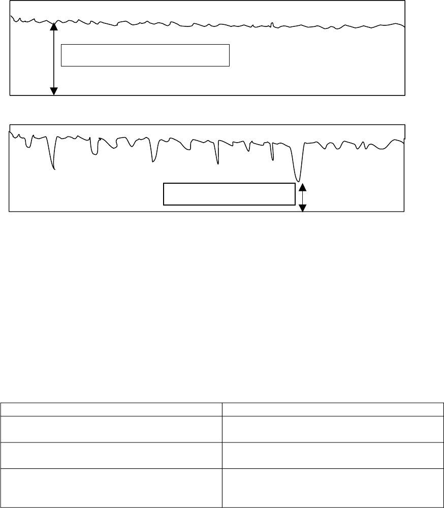
Corrosion damage may be classified according to their morphologies to be uniform (general)

corrosion or non-uniform (pitting) corrosion. When a material deteriorates with uniform

corrosion its life may be defined as the point at which the average thickness reaches a

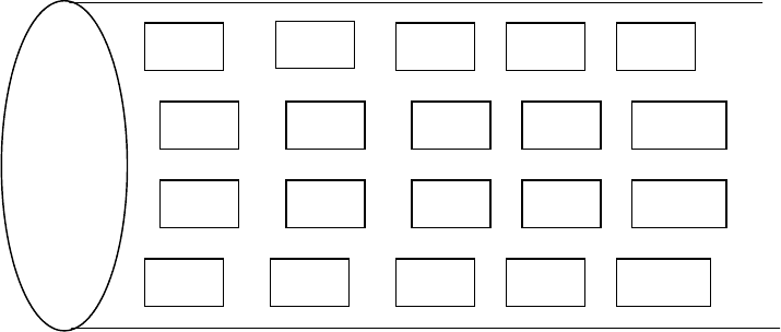
minimum allowable threshold (see Figure 9).

The upper example in Figure 9 shows an example of uniform corrosion. Due to the

uniformity of the defect, fundamental statistical distributions can be used to predict the

average wall thickness loss.

The lower surface in Figure 9 shows an example of non-uniform corrosion displaying more

localised defect penetrations. In this case considerations of the average pit depth are

inappropriate since loss of containment will result as soon as one extreme defect perforates

the material. Fundamental statistical distributions are not suitable for analysis of such cases,

and extreme value calculations are required in order to predict a maximum expected pit depth

from what will generally be sample information. The need for the use of the extreme value

distribution will be evident when the NDT data is analysed.

Extreme value data sampling differs from fundamental data sampling in that the former only

considers a set of extreme values extracted from a larger sample (as described above for each

circular ring above). Statistically the effect of this filtering (i.e. using only part of the

distribution) allows the tail of the resulting distribution to more accurately model the potential

defect extremes which may exist in the material. In practice to allow statistical integrity each

extreme value must be collected from a subset of a larger sample which in itself (i.e. the

subset) contains sufficient data to infer a parent fundamental distribution population.

Effective Thickness

Figure 9

Top: uniform corrosion, Bottom: non-uniform corrosion

Kowaka (9) has attempted to fit several types of corrosion data to different distributions, some

examples of which are in Table 1. However in most inspection situations there is little prior

knowledge of the distribution type, and therefore a full fitting operation is needed prior to any

assumptions about the distribution.

Table 1

Types of Distribution for Corrosion (from Kowaka)

Corrosion Type Distribution

Pit Depth for Carbon Steel fresh water supply Normal

pipe

Maximum Pit Depth for Petroleum Tank Extreme Value (Type 1)

Bottom Plate

Maximum Corrosion Depth beneath corrosion Extreme Value (Type 1)

product layer for carbon steel tubing for

mineral dressing slurry

4.2 DETERMINATION OF DISTRIBUTION (UNKNOWN CORROSION)

4.2.1 Collecting and Sampling the Data

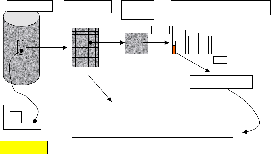
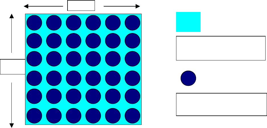
The manner in which data is collected and later analysed is represented in Figure 10. The

vessel/pipe is first divided into sample areas for inspection (often determined by the

inspection device scanner). An individual sample area (known sometimes as a patch)

contains a number of individual values of thickness or pit depth taken by the NDT device.

1 2

0.5 1.2

(patch)

Patch 3……..

Max Pit Depth 0.6……

Extreme Values

Vessel/Pipe Sample Areas

Sample

Pit Depth or Wall thickness values

DT Scanne

Figure 10

Data Collection from a vessel/pipe to produce extreme values

4.2.2 Identifying homogeneity within the vessel/pipework

As an initial step, the homogenous areas (i.e. those with similar corrosion properties) must be

identified. Statistical treatment, such as extrapolation, can only be applied with integrity to

samples which are considered to be representative of the parent populations (i.e. a larger

area). Accordingly this may result in several analyses being conducted for the vessel as a

whole.

Scanning Method

Data collection is typically (though not always) performed in a uniform manner, typically as

equally spaced measurements on a grid as depicted in the schematic below. It is important to

draw the distinction between the sample area represented by a patch of data and the effective

area scanned by the NDT probe. The sample area can be defined as the surface area of that

portion of the vessel under examination. The effective scanned area is the sum of all the areas

actually covered by the probe within the boundary of the sample area. If calculations such as

extrapolation are carried out, then the effective area should be used.

Clearly there is a direct relationship between the effective scanned area, the scan mechanism

and the resulting number of data points. By way of illustrating the relationship, Figure 11

shows a sample area of approximately 56 cm

in which 36 spot data points have been

collected using a probe of 1cm diameter. The resulting effective area scanned is about 28cm

representing about 50% of the patch area

7.5cm

7.5c

(

(0.5)

2 2

Sample (patch) area = 6 1.25 x

1.25)=56.25cm

Effective scanned area=6 x6 x

=28.27cm

Figure 11

Effective scanning Area

4.2.3 Extracting Extreme Values

Based on the NDT Equipment, its resolution (i.e. the effective area actually scanned in one

measurement recorded by the probe) and ideally, the confidence level required by the analyst,

a set of sample areas is defined and scanned. Often, in practice, this may be all of the

accessible areas, in which case the confidence level is set by the number of data points which

can be taken. The measurements are then recorded and analysed. An example of extreme

value selection of the data (which may be undertaken if prior knowledge of the corrosion

indicates pitting) is shown in Figure 10 selected from each patch. When attempting to use

extreme value analysis, it is imperative that each patch of data complies with the following

criteria:

· Each individual patch contains sufficient measurements within itself to reflect a

representative sample from the fundamental distribution. This is necessary to support the

selection of an extreme value from that patch. Literature indicates that at least 5 readings

are needed.

· the total number of extreme values that result across all patches (i.e. making up the

extreme value data as a whole) are sufficient to enable a doubly exponential (or other

extreme value) distribution to be adequately defined.

To fit distributions by matching the inspection data plotted as frequency or cumulative

distributions to the mathematical plots by trial and error (as described in 4.1) could be

extremely time consuming, and the task can be made much easier by the use of probability

plots. These are specially designed graphs which have an ordinate scale from 0 to 1, but the

intervals on the scale depend on the distribution function. If the data matches a distribution

then it will appear as a straight line. To use this method, the first step is to order the data as

above (Section 4.1). The next step is to insert this data directly on to the probability plot.

Many statistical packages have probability plots for a range of distributions included as

standard.

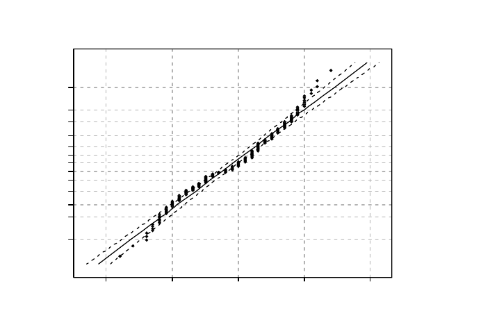
When the data is plotted, a best fit regression line of the data is also plotted. If the two

correspond, then the data matches the distribution described by the probability plot. If it

doesn’t fit then another distribution must be tried. The parameters of the distribution (i.e.

those numbers which represent the spread and location, or central tendency) are determined

from the slope of the line and its intercept with the horizontal axis.

Figure 12

Probability Plot showing fit to Normal Distribution

An immediate application of the plot is to estimate the proportion of the plant below a certain

thickness. In the probability plot this is simply read off the horizontal axis (for Figure 12, 1%

of vessel is below about 24mm thick)

23.5 24.5 25.5 26.5 27.5

Data

Percent

Max. Likelihood

Estimates:-

Mean:

StDev:

25.4mm

0.66mm