Health and Safety Executive. Guidelines for use of statistics for analysis of sample inspection of corrosion

Подождите немного. Документ загружается.

5 THE USE OF INSPECTION DATA

5.1 GENERAL COMMENTS ON DATA COLLECTION

5.1.1 Manual Ultrasonic Thickness Gauge/A-Scan

Where the data collected by ultrasonic thickness gauge or A-Scan equipment is sampled from

pre-determined locations on a component, the data may be analysed for an underlying

distribution. One exception to this is when the data is in a very close grid, in which case a it

is advisable to carry out a spatial analysis similar to that for scanned UT systems (see below).

Alternatively, where the ultrasonic procedure is that of scanning individual portions of a

vessel and reporting only the minimum thickness seen in each portion, then extreme value

data is being collected and the extreme value approach can be applied directly.

5.1.2 Automatic Scanned Systems

Scanning UT systems collect a large amount of data in a grid pattern. This data is taken

offline of the NDT system for analysis. The raw data is suitable for underlying distribution

analysis, subject to the individual readings being independent of each other. This can be

tested by applying a spatial autocorrelation function to the data. This process is described in

Appendix A.

If the autocorrelation distance is greater than the distance between readings then the readings

used must be separated by at least the former distance. This involves grouping the data. An

extreme value analysis can be implemented by taking the minimum value of each group.

5.2 DETERMINATION OF CORROSION RATE - CURRENT PRACTICE

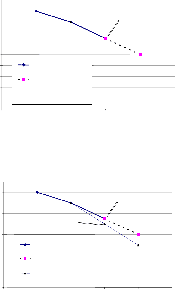
Current methods of corrosion rate determination and life prediction tend to rely on a

simplistic treatment of thickness gauge readings. Usually the minimum thicknesses or the

thickness at particular locations at the last two inspections are taken and the prediction is a

linear extrapolation (as in Figure 13).

ll ( )

ion

ini i

Wa Thickness mm

Th ckness Measurements

Predict

Measured M mum Th ckness

0 5 10 15 20

Time (years)

Figure 13

Simple corrosion rate method

If the appropriate measurement is not made in each case, perhaps because the actual minimum

has not been found in a scan, then the estimation of corrosion rate may be inaccurate. Figure

14 shows what can happen in this case.

( )Wall Thickness mm

Thickness Measurements

Prediction

Actual rate of corrosion

Measured Minimum Thickness

Actual Minimum Thickness

0 5 10 15 20

Time (years)

Figure 14

Illustration of Errors in Corrosion Rate Estimation caused by Inspection Errors

Where many readings are taken in an inspection survey, the use of minimum thicknesses or

even individual thickness readings at a particular location can result in similar errors in the

estimation of corrosion rate.

Figure 15 shows how this error can occur.

02 46 81012

( )Wall Thickness mm

Corrosion Rate estimated

from minimum readings

Mean Corrosion Rate

Time

Figure 15

Methods for estimating corrosion rate

These problems are exacerbated if there is pitting corrosion, since individual readings are

unlikely to be representative of the minimum thickness, and since errors are much more likely

in the inspection method (11,12). A source of error in the corrosion rate might also occur if

any random scatter in the inspection method is reduced in successive inspections (for example

by using improved techniques). In Figure 15 a lower corrosion rate is estimated by using the

minimum thickness measurements than by using the mean value.

Statistical methods can help to solve these problems; sometimes even the simplest method

will improve the likely accuracy of corrosion rate estimation.

5.3 SUGGESTED ANALYSIS METHODS – NORMAL DISTRIBUTION

5.3.1 Determination of Corrosion Rate

It is currently common practice to estimate the corrosion rate from the minimum wall

thickness measurement from each inspection, rather than from the mean. When the corrosion

is uniform this procedure is especially prone to NDT measurement errors, because the

minimum wall thickness simply reflects the worst undersizing of the wall thickness rather

than any genuine variation due to the corrosion itself. For uniform corrosion, regression

analysis is preferable. It is therefore recommended that multiple readings be taken for each

case, the average calculated, and this value used to estimate the corrosion rate. This will then

yield not only a best estimate of the trend in the data, but can also be used to:

· check that the magnitude of any random measurement errors about this trend is as

expected

· if required, estimate confidence limits on both the present and future corrosion.

Simple regression analysis is now available, not only within statistical software, but also

within most spreadsheet packages. Failing this the rate can be estimated from the difference

between the maximum loss of wall in the most recent inspection and the minimum loss of

wall in the previous inspection(s). This will, in most cases, lead to a conservative estimate of

corrosion rate.

5.3.2 Proportion below thickness

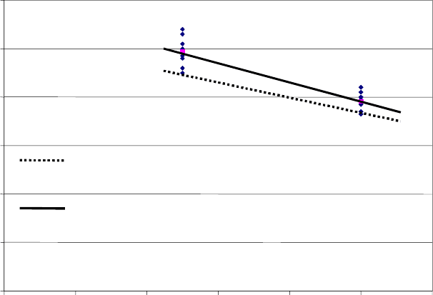
The proportion below a certain thickness can be estimated from the probability graph. The

thickness required is obtained from the horizontal axis, and the percentage of the area below

this thickness is given by the probability reading corresponding to this thickness and the best

fit line.

In Figure 12 for example the solid line illustrates a fitted distribution, while the dashed lines

represent the 95% confidence limits. In this case, it can be seen that very little corrosion has

occurred. The plot indicates, for instance, that ~1% of the thicknesses fall below 24mm. In

general, the normal distribution gives a reasonably good fit to the data, but there appears to be

a trend for the data to fall slightly below the fitted line for thicknesses less than about 24mm.

This suggests that any predictions based on the fitted line within this thickness range will tend

to be slightly conservative.

5.3.3 Area Extrapolation for Minimum Thickness Estimation (underlying

distributions)

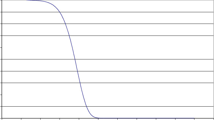
This is achieved by the use of the survivor function (Figure 7). It can be established that the

survivor function raised to the power of the ratio of total extrapolated area to inspection area

gives the survivor function of the minimum thickness over the extrapolated area. Suppose

that the survivor function in Figure 7 represents data from, for example, 1/100 of the total

plant area, then in order to estimate the minimum value over the whole area, the probability

values in Figure 7 are taken to the power of 100. This produces the distribution of minimum

thickness in Figure 16, which shows that the probability that the minimum wall thickness over

the whole area being less than 4.6mm is around 10%.

Where this ratio gets very large, the distribution of minimum thickness approximates to an

extreme value distribution (see, for example, Gumbel (4))

Survivor^100

0.9

0.8

0.7

0.6

0.5

0.4

0.3

0.2

0.1

4.3 4.4 4.5 4.6 4.7 4.8 4.9 5 5.1 5.2 5.3 5.4

Wall Thickness (mm)

Figure 16

Survivor Function of Minimum Thickness over 100 times Area as Figure 7

5.4 EXTREME VALUE FITTED DATA (TYPE 1 DISTRIBUTION)

5.4.1 Probability Plot

If the underlying distribution is an extreme value one, then it is possible that the corrosion is

pitting. In this case the probability graph can be used directly to obtain an estimation of

minimum thickness or maximum pit depth. The extreme values can be obtained by taking

data in patches (either by scanning an area and getting the minimum wall thicknesses in each

area, or by collecting all the data from an area, dividing it into patches and using the minima

from these patches, or by selecting the maximum pit sizes from a given area).

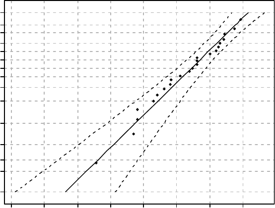
Figure 17 shows an example. The inspection area or patch was 0.03m

and the minimum

thicknesses from a number of them are shown as plotted points.

The fitted line indicates, for

instance, that if a 0.03 m

patch is randomly selected from the whole area then there is a 5%

probability of the minimum thickness in this patch being less than 11mm. The plotted 95%

confidence limits (shown dashed in Figure 17) can also be used as an aid to judgement. In this

case, the data show a good fit to an extreme value distribution.

Statistical software can then be used to estimate the location and scale parameters (m and s)

of the distribution, as shown in the top right of Figure 17.

Max imum L ike lih oo d

Percent

Estimates:-

Location: 13.7764

Scale: 0.900694

8 9 10 11 12 13 14 15

Data

Figure 17

Example of Extreme Value Distribution

5.4.2 Area Extrapolation (Extreme Value Type 1)

The method described by Gumbel gives an estimation of maximum pit size. The maximum

pit sizes from a given area are ordered, then plotted on the extreme value probability paper.

An example is given in Figure 18. The right hand axis shows the number of data points (i.e.

the number of maximum pit depths each of which corresponds to a given area). In this case

10 points have been measured. If we wished to estimate the maximum pit depth for 500

measurements we refer to the 500 on the right hand axis and the line at Point A. Point B

corresponds to the minimum thickness over the extrapolated area.

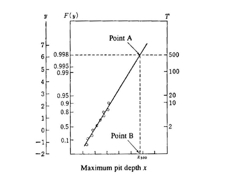
Figure 18

Return period method of extrapolating over area

(from Kowaka (9))

Note that this method does not include confidence limits on the estimation, nor does it

produce the distribution of minimum thicknesses that is needed for reliability analysis. To

achieve these the method described by Schneider et al (13) should be used, and the work of

Reiss and Thomas (14) and Laycock (15) from which this is derived also studied.

5.5 DETERMINATION OF CORROSION RATE

When a Type 1 Extreme Value distribution has been identified, estimation of corrosion rate

can be carried out using the probability plot, as described by Kowaka (9) (Figure 19). In this

case it can be seen that the graph shifts across the thickness axis in time. The rate of

corrosion can be estimated from the shift. The method works provided that the slope of the

graph does not change between inspections. Should that occur, different parts of the

component are corroding at different rates. Modelling of the distribution of the corrosion rate

in this situation is beyond the scope of this document.

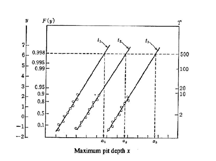
Figure 19

Corrosion Rate from Extreme Value Probability Plot

(from Kowaka (9))

5.6 NUMBER OF SAMPLES NEEDED (EACH CASE)

5.6.1 UT Methods

UT methods fall into three categories for corrosion inspection as mentioned in 5.1 above.

1. Sample readings with thickness gauges

2. Sample area scans with A-Scan instruments for minima within an area

3. Automated scans with recorded readings in a grid.

The choice of UT method depends on cost and the quality and quantity of data required. The

cost will increase in particular with the deployment of automated systems, although all

methods require the removal of coatings.

It should be pointed out that standard UT measurements are the only ones which will give a

direct thickness reading of a small area, and are therefore the only ones suitable for

measurement of pitting (although there are some restrictions) (11,12). They are also usually

significantly more sensitive to variations in wall thickness (e.g. ~0.1mm) than the alternative

methods.

5.7 CHOICE OF LOCATION

When using ultrasonic inspection in an unknown situation it is generally preferable to

determine at some stage whether pitting corrosion is occurring. This can usually be identified

by an experienced operator with manual equipment, or more positively by a scanning system.

The inspection locations should ensure that possible different cases of corrosion are inspected

and checked to see if different statistics apply. Each Case corresponds to a potentially

different corrosion environment, and may result from differing:

· Materials

· Corrosion product/chemistry

· Temperature

· Flow rate

· Presence of inhibitor

· Component geometry, e.g. orientation, level or clock position (for horizontal pipe)

· Fluid Composition

· Presence of Contaminants

Each Case must be treated separately to determine the sample numbers needed. In principle

within those areas the data collection can be at any randomly selected points or areas.

The choice of locations for inspection made on a risk-based or experience-based

methodology, targeted at ‘hot spots’, is not within the scope of this document.

5.7.1 Other methods

While this document is primarily associated with the use of standard ultrasonic methods, it is

recognised that other methods do exist for corrosion inspection and it may be necessary to

consider these as options for planning an inspection. A table of the alternative methods is

given below together with their main characteristics and difficulties. For statistical analysis

the other methods may sometimes produce thickness measurements which appear similar to

UT. It should be noted that techniques which have a large footprint are not capable of

providing the detailed information necessary for sampling. For generic statistical reasons, the

data is more likely to fit a normal distribution for general corrosion whatever the surface

morphology.

Method Main application area Possible restrictions

Creeping Head Wave Under clamp inspection Coatings / qualitative measurement

/ lack of internal-external

discrimination

Long Range Low Screening / road crossings / Some coatings / sensitive to loss of

Frequency Ultrasonics large areas / difficult access overall cross section / lack of

internal-external discrimination

Pulsed Eddy Current Under insulation Large footprint / proximity of other

objects / lack of internal-external

discrimination

Not welds

Magnetic Flux Leakage Fast screening / some special Thickness limitation / internal-

methods for small diameter external discrimination difficult

pipe Not welds

SLOFEC Fast measurement Scaling output to thickness

Thickness variation signals from

other causes

X Ray Under insulation Radiation hazard

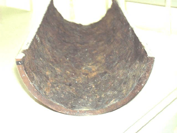
6 CASE STUDY: FAILED OIL PIPE

A 100mm dia. pipe carrying crude oil had been supplied to the project by an operator. This

had been removed from service due to a leakage failure. The total length of the pipe in service

was 25metres. A sample of the pipe (Figure 19a) was investigated. This gives a total of 16

inspected areas, which is extrapolated to 1250 areas.

Figure 19a

Corroded Pipe Sample

The pipe sample shown was divided into 16 areas and the minimum ultrasonic thickness

(measured from the outside) was ascertained in each area by a manual search for the

minimum thickness.

The ordered results were:

3.33 4.19

3.63 4.26

3.8 4.34

3.82 4.77

3.82

3.92

3.98

4.04

4.06

4.1

4.13