Hull J.C. Risk management and Financial institutions

Подождите немного. Документ загружается.

150 Chapter 6

tools for specifying the correlation structure between variables—even

when the distributions of the variables are not normal.

We start by considering a bivariate normal distribution, where there are

only two variables, V

and V

. Suppose that we know V

has some

value Conditional on this, the value of V

is normal with mean

and standard deviation

Here and are the unconditional means of V

and V

; and are

their unconditional standard deviations; and is the coefficient of cor-

relation between V

and V

. Note that the expected value of V

condi-

tional on V

is linearly dependent on the value of V

. This corresponds to

Figure 6.1a. Also the standard deviation of V

conditional on the value of

is the same for all values of V

Generating Random Samples from Normal Distributions

Most programming languages have routines for sampling a random

number between 0 and 1 and many have routines for sampling from a

normal distribution.

If no routine for sampling from a standardized

normal distribution is readily available, an approximate random sample

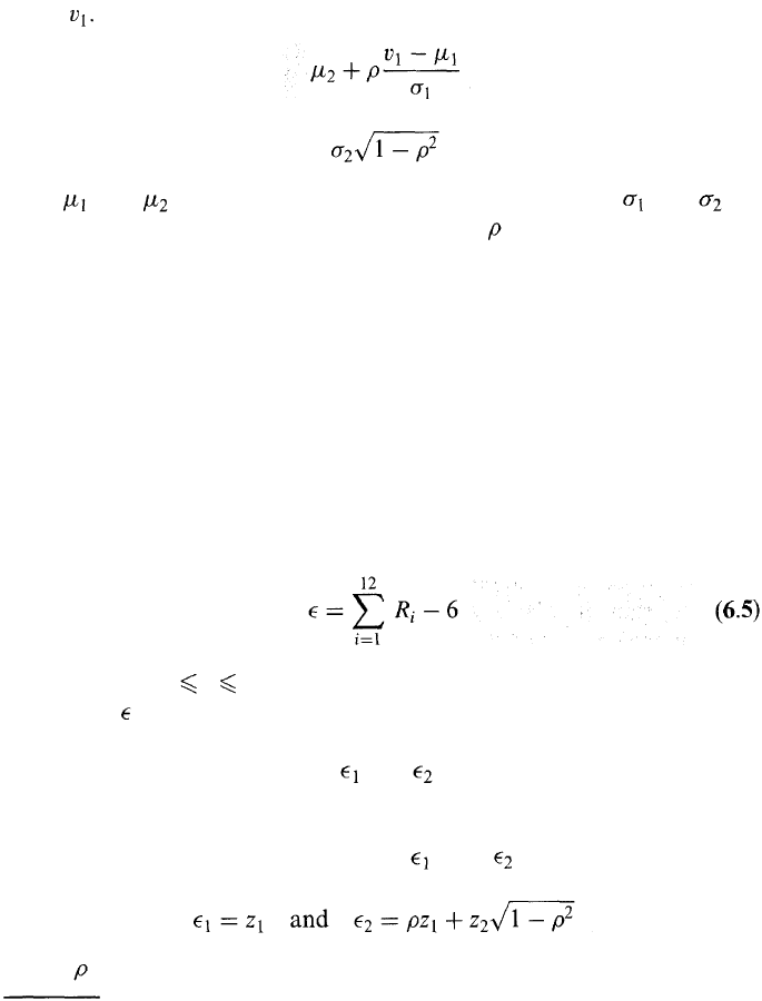
can be calculated as

where the R

(1 i 12) are independent random numbers between 0

and 1, and is the required sample. This approximation is satisfactory for

most purposes.

When two correlated samples and from bivariate distributions are

required, an appropriate procedure is as follows. Independent samples z

and z

from a univariate standardized normal distribution are obtained as

just described. The required samples and are then calculated as

follows:

where is the coefficient of correlation.

In Excel the instruction =NORMSINV(RAND()) gives a random sample from a

normal distribution.

Correlations and Copulas

151

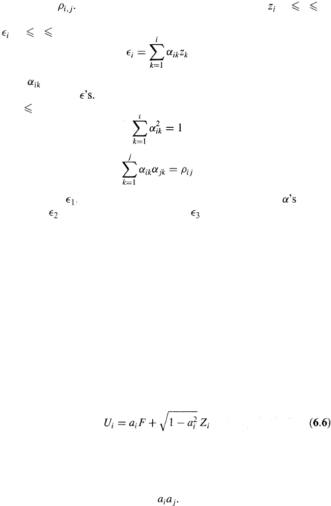
Consider next the situation where we require n correlated samples from

normal distributions and the coefficient of correlation between sample i

and sample j is We first sample n independent variables (1 i n)

from univariate standardized normal distributions. The required samples

are (1 i n), where

and the are parameters chosen to give the correct variances and

correlations for the

For 1 j < i, we have

and, for all j < i,

The first sample, , is set equal to z\. These equations for the can be

solved so that is calculated from z

and z

, is calculated from z

, z

and

, and so on. The procedure is known as the Cholesky decomposition.

If we find ourselves trying to take the square root of a negative number

when using the Cholesky decomposition, the variance-covariance matrix

assumed for the variables is not internally consistent. As explained in

Section 6.2, this is equivalent to saying that the matrix is not Positive-

semidefinite.

Factor Models

Sometimes the correlations between normally distributed variables are

defined using a factor model. Suppose that U

,... ,U

have standard

normal distributions (i.e., normal distributions with mean 0 and standard

deviation 1). In a one-factor model each U

has a component dependent on

a common factor F and a component that is uncorrelated with the other

variables. Formally,

where F and the Z

have a standard normal distributions and a

is a

constant between —1 and +1. The Z

are uncorrelated with each other

and uncorrelated with F. In this model all the correlation between U

and

arises from their dependence on the common factor F. The coefficient

of correlation between U

and U

152

Chapter 6

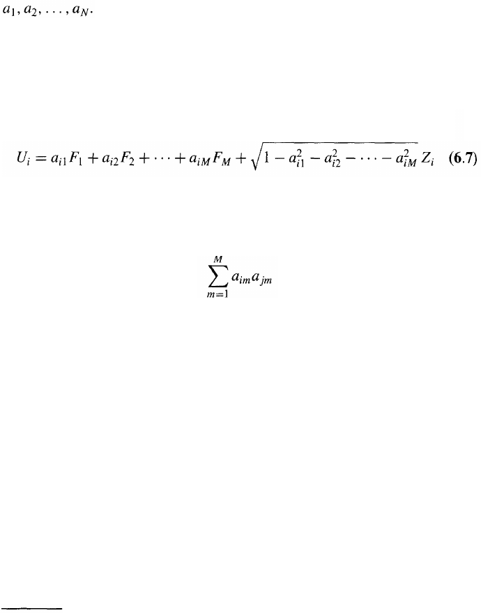
The advantage of a one-factor model is that it imposes some structure

on the correlations. Without assuming a factor model the number of

correlations that have to be estimated for the N variables is N(N — l)/2.

With the one-factor model we need only estimate N parameters:

An example of a one-factor model from the world of

investments is the capital asset pricing model, where the return on a stock

has a component dependent on the return from the market and an

idiosyncratic (nonsystematic) component that is independent of the return

on other stocks (see Section 1.1).

The one-factor model can be extended to a two-, three-, or M-factor

model. In the M-factor model,

The factors F

, F

,..., F

have uncorrelated standard normal distribu-

tions and the Z

are uncorrelated both with each other and with the F's.

In this case the correlation between U

and U

6.4 COPULAS

Consider two correlated variables V\ and V

.The marginal distribution of

(sometimes also referred to as the unconditional distribution) is its

distribution assuming we know nothing about V

; similarly, the marginal

distribution of V

is its distribution assuming we know nothing about V

Suppose we have estimated the marginal distributions of V

and V

. How

can we make an assumption about the correlation structure between the

two variables to define their joint distribution?

If the marginal distributions of V

and V

are normal, an assumption

that is convenient and easy to work with is that the joint distribution of

the variables is bivariate normal.

Similar assumptions are possible for

some other marginal distributions. But often there is no natural way of

defining a correlation structure between two marginal distributions. This

is where copulas come in.

Although this is a convenient assumption it is not the only one that can be made. There

are many other ways in which two normally distributed variables can be dependent on

each other. See, for example, Problem 6.11.

Correlations and Copulas 153

(a)

(b)

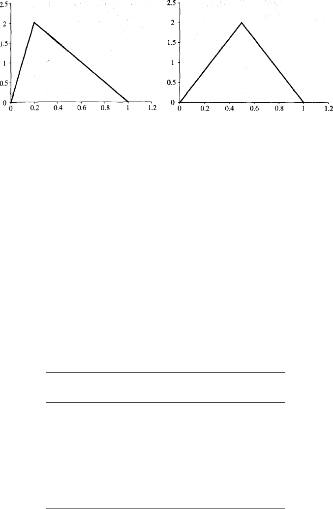
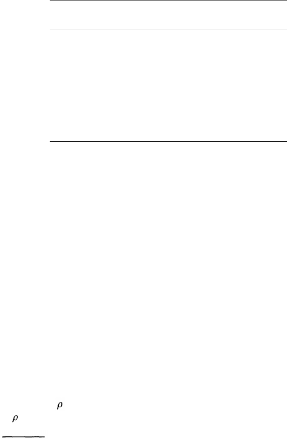
Figure 6.2 Triangular distributions for (a) V

and (b) V

As an example of the application of copulas, suppose that the marginal

distributions of V

and V

are the triangular probability density functions

shown in Figure 6.2. Both variables have values between 0 and 1. The

density function for V

peaks at 0.2, and the density function for V

peaks

at 0.5. For both density functions, the maximum height is 2.0. To use what

is known as a Gaussian copula, we map V

and V

into new variables U

and

that have standard normal distributions. (A standard normal distribu-

tion is a normal distribution with mean 0 and standard deviation 1.) The

mapping is effected on a percentile-to-percentile basis. The 1-percentile

point of the V

distribution is mapped to the 1-percentile point of the U

distribution; the 10-percentile point of the V

distribution is mapped to the

10-percentile point of the U

distribution; and so on. The variable V

mapped into U

in a similar way. Table 6.1 shows how values of V

are

Table 6.1 Mapping of V

, which has the triangular

distribution in Figure 6.2a, to U

, which has a standard

normal distribution.

value

0.1

0.2

0.3

0.4

0.5

0.6

0.7

0.8

0.9

Percentile

of distribution

5.00

20.00

38.75

55.00

68.75

80.00

88.75

95.00

98.75

value

-1.64

-0.84

-0.29

0.13

0.49

0.84

1.21

1.64

2.24

154

Chapter 6

Table 6.2 Mapping of V

, which has the triangular

distribution in Figure 6.2b, to U

, which has a standard

normal distribution.

value

0.1

0.2

0.3

0.4

0.5

0.6

0.7

0.8

0.9

Percentile

of distribution

2.00

8.00

18.00

32.00

50.00

68.00

82.00

92.00

98.00

value

-2.05

-1.41

-0.92

-0.47

0.00

0.47

0.92

1.41

2.05

mapped into values of U

and Table 6.2 how values of V

are mapped into

values of U

. Consider the V

=0.1 calculation in Table 6.1. The cumula-

tive probability that V

is less than 0.1 is (by calculating areas of triangles)

0.5 x 0.1 x 1 = 0.05, or 5%. The value 0.1 for V

therefore gets mapped to

the 5-percentile point of the standard normal distribution. This is —1.64.

The variables U

and U

have normal distributions. We assume that

they are jointly bivariate normal. This in turn implies a joint distribution

and a correlation structure between V

and V

. The essence of copulas is

therefore that, instead of defining a correlation structure between V

and

directly, we do so indirectly. We map V

and V

into other variables

which have "well-behaved" distributions and for which it is easy to define

a correlation structure.

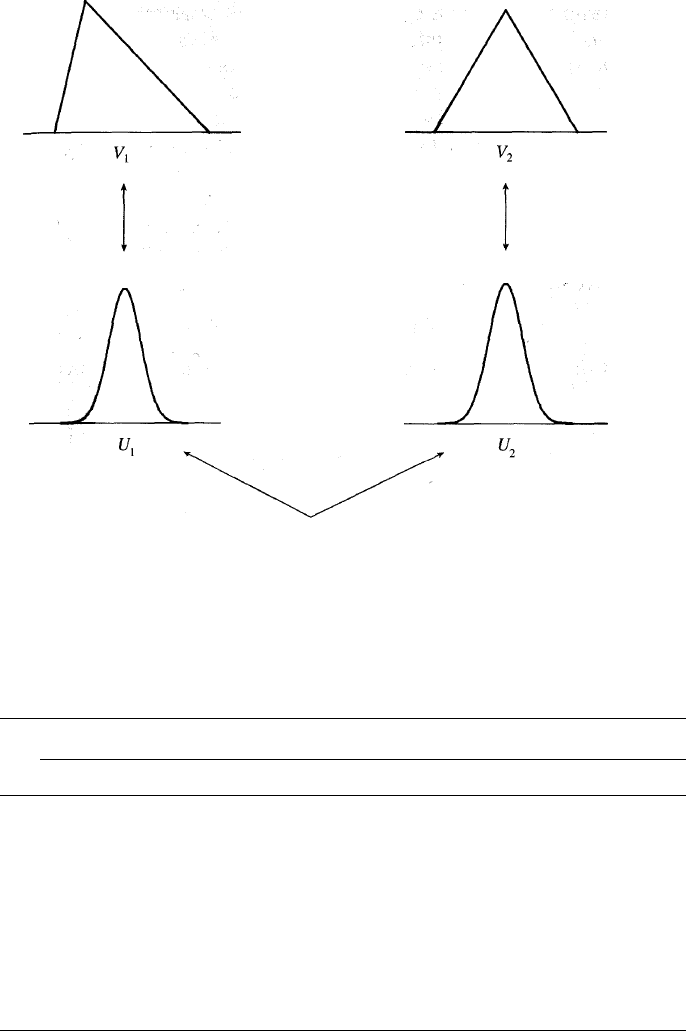
The way in which a copula defines a joint distribution is illustrated in

Figure 6.3. Let us assume that the correlation between U

and U

is 0.5.

The joint cumulative probability distribution between V

and V

is shown

in Table 6.3. To illustrate the calculations, consider the first one where we

are calculating the probability that V

< 0.1 and V

< 0.1. From Tables 6.1

and 6.2, this is the same as the probability that U

< —1.64 and

< -2.05. From the cumulative bivariate normal distribution, this is

0.006 when = 0.5.

(The probability would be only 0.02 x 0.05 = 0.001

if =0.)

It can be calculated using Excel: NORMSINV(0.05) = -1.64.

An Excel function for calculating the cumulative bivariate normal distribution can be

found on the author's website: www.rotman.utoronto.ca/~hull.

Correlations and Copulas

155

One-to-one

mappings

Correlation assumption

Figure 6.3 The way in which a copula model defines a joint distribution.

Table 6.3 Cumulative joint probability distribution for V

and V

in a

Gaussian copula model. Correlation parameter =0.5. Table shows the joint

probability that V

and V

are less than the specified values.

0.1

0.2

0.3

0.4

0.5

0.6

0.7

0.8

0.9

0.1

0.006

0.013

0.017

0.019

0.020

0.2

0.017

0.043

0.061

0.071

0.076

0.078

0.079

0.080

0.3

0.028

0.081

0.124

0.149

0.164

0.173

0.177

0.179

0.180

0.4

0.037

0.120

0.197

0.248

0.281

0.301

0.312

0.318

0.320

0.5

0.044

0.156

0.273

0.358

0.417

0.456

0.481

0.494

0.499

0.6

0.048

0.181

0.331

0.449

0.537

0.600

0.642

0.667

0.678

0.7

0.049

0.193

0.364

0.505

0.616

0.701

0.760

0.798

0.816

0.8

0.050

0.198

0.381

0.535

0.663

0.763

0.837

0.887

0.913

0.9

0.050

0.200

0.387

0.548

0.683

0.793

0.877

0.936

0.970

156 Chapter 6

The correlation between U

and U

is referred to as the copula correl-

ation. This is not, in general, the same as the correlation between V

and

. Since U

and U

are bivariate normal, the conditional mean of U

linearly dependent on U

and the conditional standard deviation of U

constant (as discussed in Section 6.3). However, a similar result does not

in general apply to V

and V

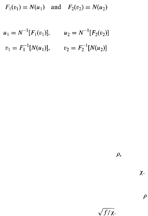
Expressing the Approach Algebraically

For a more formal description of the Gaussian copula approach, suppose

that F

and F

are the cumulative marginal probability distributions of V

and V

. We map V

= v

to U

= u

and V

= v

to U

= u

, where

and N is the cumulative normal distribution function. This means that

and

The variables U

and U

are then assumed to be bivariate normal. The

key property of a copula model is that it preserves the marginal distribu-

tions of V

and V

(however unusual these may be) while defining a

correlation structure between them.

Other Copulas

The Gaussian copula is just one copula that can be used to define a

correlation structure between V

and V

. There are many other copulas

leading to many other correlation structures. One that is sometimes used

is the Student t-copula. This works in the same way as the Gaussian

copula except that the variables U

and U

are assumed to have a

bivariate Student t-distribution. To sample from a bivariate Student

t-distribution with f degrees of freedom and correlation we proceed

as follows:

1. Sample from the inverse chi-square distribution to get a value (In

Excel, the CHIINV function can be used. The first argument is

RAND() and the second is f.)

2. Sample from a bivariate normal distribution with correlation as

described in Section 6.3.

3. Multiply the normally distributed samples by

Correlations and Copulas 157

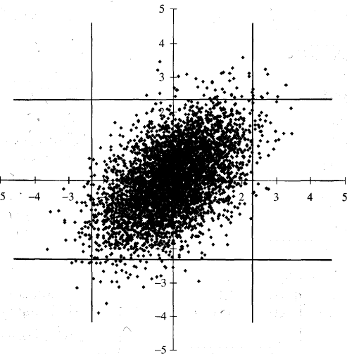
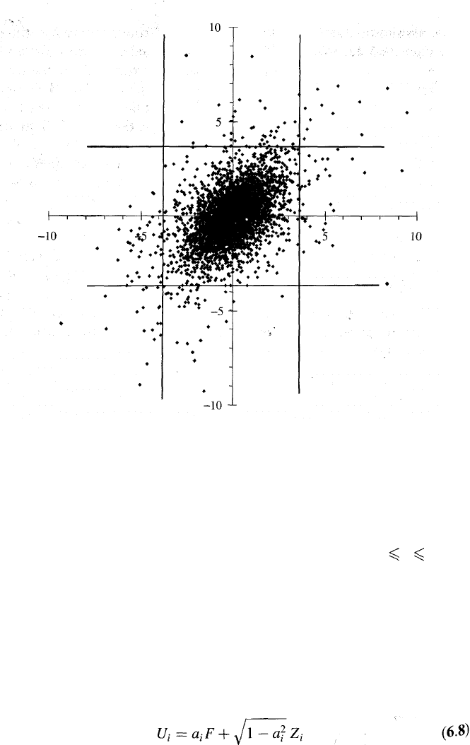
Figure 6.4 shows plots of 5000 random samples from a bivariate normal,

while Figure 6.5 does the same for the bivariate Student t. The correlation

parameter is 0.5 and the number of degrees of freedom for the Student t

is 4. Define a "tail value" of a distribution as a value in the left or right

1 % tail of the distribution. There is a tail value for the normal distribu-

tion when the variable is greater than 2.33 or less than —2.33. Similarly

there is a tail value in the t-distribution when the value of the variable is

greater than 3.75 or less than -3.75. Vertical and horizontal lines in the

figures indicate when tail values occur. The figures illustrate that it is more

common for both variables to have tail values in the bivariate t-distribu-

tion than in the bivariate normal distribution. To put this another way,

the tail correlation is higher in a bivariate t-distribution that in a bivariate

normal distribution. We made the point earlier that correlations between

market variables tend to increase in extreme market conditions so that

Figure 6.1c is sometimes a better description of the correlation structure

between two variables than Figure 6.1a. This has led some researchers to

argue that the Student t-copula provides a better description of the joint

behavior of market variables than the Gaussian copula.

Figure 6.4 5000 random samples from a bivariate normal distribution.

158

Chapter 6

Figure 6.5 5000 random samples from a bivariate Student t-distribution.

Multivariate Copulas

Copulas can be used to define a correlation structure between more than

two variables. The simplest example of this is the multivariate Gaussian

copula. Suppose that there are N variables, V

,...,

, and that we

know the marginal distribution of each variable. For each i (1 i N), we

transform V

into U

where U

has a standard normal distribution (the

transformation is effected on a percentile-to-percentile basis as above). We

then assume that the U

have a multivariate normal distribution.

A Factor Copula Model

In multivariate copula models, analysts often assume a factor model for

the correlation structure between the U

. When there is only one factor,

equation (6.6) gives

Correlations and Copulas

159

where F and the Z

have standard normal distributions. The Z

are

uncorrelated with each other and uncorrelated with F. Other factor copula

models are obtained by choosing F and the Z

to have other zero-mean

unit-variance distributions. For example, if Z

is normal and F has a

Student t-distribution, we obtain a multivariate Student t-distribution

for U

. These distributional choices affect the nature of the dependence

between the variables.

6.5 APPLICATION TO LOAN PORTFOLIOS

We now present an application of the one-factor Gaussian copula that

will prove useful in understanding the Basel II capital requirements in

Chapter 7. Consider a portfolio of N companies. Define T

(1 i N) as

the time when company i defaults. (We assume that all companies will

default eventually—but that the default time may be a long time, perhaps

even hundreds of years, in the future.) Denote the cumulative probability

distribution of 7} by Q

In order to define a correlation structure between the T

using the one-

factor Gaussian copula model, we map, for each i, T

to a variable U

that

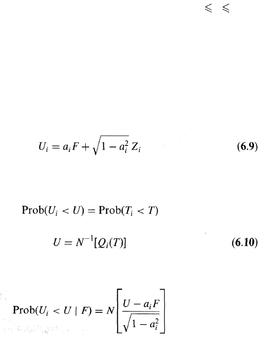
has a standard normal distribution on a percentile-to-percentile basis. We

assume the factor model in equation (6.8) for the correlation structure

between the U

where the variables F and Z

have independent standard normal distribu-

tions. The mappings between the U

and T

imply

when

From equation (6.9), the probability that U

< U conditional on the

factor value F is