Jackson S.L. Research Methods and Statistics: A Critical Thinking Approach
Подождите немного. Документ загружается.


182
■ ■
CHAPTER 7
Confidence Intervals Based
on the z Distribution
In this text, hypothesis tests such as the previously described z test are
the main focus. However, sometimes social and behavioral scientists use
estimation of population means based on confidence intervals rather than
statistical hypothesis tests. For example, imagine that you want to estimate
a population mean based on sample data (a sample mean). This differs from
the previously described z test in that we are not determining whether the
sample mean differs significantly from the population mean; rather, we are
estimating the population mean based on knowing the sample mean. We can
still use the area under the normal curve to accomplish this—we simply use
it in a slightly different way.
Let’s use the previous example in which we know the sample mean
weight of children enrolled in athletic after-school programs (
X 86),
(17), and the sample size (N 100). However, imagine that we do not
know the population mean (). In this case, we can calculate a confidence
interval based on knowing the sample mean and . A confidence interval is
confidence interval An
interval of a certain width which
we feel confident will contain .
confidence interval An
interval of a certain width which
we feel confident will contain .
IN REVIEW The z Test (Part II)
CONCEPT DESCRIPTION EXAMPLE
One-Tailed z Test A directional inferential test in which a prediction is made H
a
:
0
1
that the population represented by the sample will be or
either above or below the general population. H
a
:
0
1
Two-Tailed z Test A nondirectional inferential test in which the prediction H
a
:
0
1
is made that the population represented by the sample
will differ from the general population, but the direction
of the difference is not predicted.
Statistical Power The probability of correctly rejecting a false H
0
. One-tailed tests are
more powerful;
increasing sample
size increases power.
CRITICAL
THINKING
CHECK
7.4
1. Imagine that I want to compare the intelligence level of psychol-
ogy majors with the intelligence level of the general population of
college students. I predict that psychology majors will have higher
IQ scores. Is this a one- or two-tailed test? Identify H
0
and H
a
.
2. Conduct the z test for the preceding example. Assume that
100, 15,
X 102.75, and N 60. Should we reject H
0
or fail to reject H
0
?
10017_07_ch7_p163-201.indd 182 2/1/08 1:24:54 PM
Hypothesis Testing and Inferential Statistics
■ ■
183
an interval of a certain width, which we feel “confident” will contain . We
want a confidence interval wide enough that we feel fairly certain it contains
the population mean. For example, if we want to be 95% confident, we want
a 95% confidence interval.
How can we use the area under the standard normal curve to determine
a confidence interval of 95%? We use the area under the normal curve to
determine the z-scores that mark off the area representing 95% of the scores
under the curve. If you consult Table A.2 again, you will find that 95% of
the scores will fall between ±1.96 standard deviations above and below the
mean. Thus, we could determine which scores represent ±1.96 standard
deviations from the mean of 86. This seems fairly simple, but remember
that we are dealing with a distribution of sample means (the sampling
distribution) and not with a distribution of individual scores. Thus, we must
convert the standard deviation () to the standard error of the mean (
X
the
standard deviation for a sampling distribution) and use the standard error of
the mean in the calculation of a confidence interval. Remember, we calculate
X
by dividing by the square root of N.
X
17
______
____
100
17
___
10
1.7
We can now calculate the 95% confidence interval using the following
formula:
CI
X ± z(
X
)
where
X the sample mean
X
the standard error of the mean
z the z-score representing the desired confidence interval
CI 86 ± 1.96(1.7)
86 ± 3.332
82.668 89.332
Thus, the 95% confidence interval ranges from 82.67 to 89.33. We would con-
clude, based on this calculation, that we are 95% confident that the popula-
tion mean lies within this interval.
What if we want to have greater confidence that our population mean
is contained in the confidence interval? In other words, what if we want to
be 99% confident? We would have to construct a 99% confidence interval.
How would we go about doing this? We would do exactly what we did for
the 95% confidence interval. First, we would consult Table A.2 to determine
what z-scores mark off 99% of the area under the normal curve. We find that
z-scores of ±2.58 mark off 99% of the area under the curve. We then apply
the same formula for a confidence interval used previously.
CI
X ± z(
X
)
CI 86 ± 2.58(1.7)
86 ± 4.386
81.614 90.386
10017_07_ch7_p163-201.indd 183 2/1/08 1:24:55 PM

184
■ ■
CHAPTER 7
Thus, the 99% confidence interval ranges from 81.61 to 90.39. We would con-
clude, based on this calculation, that we are 99% confident that the popula-
tion mean lies within this interval.
Typically, statisticians recommend using a 95% or a 99% confidence inter-
val. However, using Table A.2 (the area under the normal curve), you could
construct a confidence interval of 55%, 70%, or any percentage you desire.
It is also possible to do hypothesis testing with confidence intervals.
For example, if you construct a 95% confidence interval based on knowing
a sample mean and then determine that the population mean is not in the
confidence interval, the result is significant. For example, the 95% confidence
interval we constructed earlier of 82.67 89.33 did not include the actual
population mean reported earlier in the chapter ( = 90). Thus, there is less
than a 5% chance that this sample mean could have come from this popula-
tion—the same conclusion we reached when using the z test earlier in the
chapter.
The t Test: What It Is and What It Does
The t test for a single sample is similar to the z test in that it is also a para-
metric statistical test of the null hypothesis for a single sample. As such, it
is a means of determining the number of standard deviation units a score is
from the mean () of a distribution. With a t test, however, the population
variance is not known. Another difference is that t distributions, although
symmetrical and bell-shaped, do not fit the standard normal distribution.
This means that the areas under the normal curve that apply for the z test do
not apply for the t test.
Student’s t Distribution
The t distribution, known as Student’s t distribution, was developed by
William Sealey Gosset, a chemist who worked for the Guinness Brewing
Company of Dublin, Ireland, at the beginning of the 20th century. Gosset
noticed that for small samples of beer (N 30) chosen for quality-control
testing, the sampling distribution of the means was symmetrical and bell-
shaped but not normal. In other words, with small samples, the curve was
symmetrical, but it was not the standard normal curve; therefore, the pro-
portions under the standard normal curve did not apply. As the size of the
samples in the sampling distribution increased, the sampling distribution
approached the normal distribution, and the proportions under the curve
became more similar to those under the standard normal curve. He eventu-
ally published his finding under the pseudonym “Student,” and with the
help of Karl Pearson, a mathematician, he developed a general formula for
the t distributions (Peters, 1987; Stigler, 1986; Tankard, 1984).
We refer to t distributions in the plural because unlike the z distribution,
of which there is only one, the t distributions are a family of symmetrical
distributions that differ for each sample size. As a result, the critical value
t test A parametric inferen-
tial statistical test of the null
hypothesis for a single sample
where the population variance
is not known.
t test A parametric inferen-
tial statistical test of the null
hypothesis for a single sample
where the population variance
is not known.
Student’s t distribution
A set of distributions that,
although symmetrical and
bell-shaped, are not normally
distributed.
Student’s t distribution
A set of distributions that,
although symmetrical and
bell-shaped, are not normally
distributed.
10017_07_ch7_p163-201.indd 184 2/1/08 1:24:55 PM
Hypothesis Testing and Inferential Statistics
■ ■
185
indicating the region of rejection changes for samples of different sizes.
As the size of the samples increases, the t distribution approaches the z or
normal distribution. Table A.3 in Appendix A provides the critical values
(t
cv
) for both one- and two-tailed tests for various sample sizes and alpha
levels. Notice, however, that although we have said that the critical value
depends on sample size, there is no column in the table labeled N for sam-
ple size. Instead, there is a column labeled df, which stands for degrees of
freedom—the number of scores in a sample that are free to vary. The degrees
of freedom are related to the sample size. For example, assume that you are
given six numbers: 2, 5, 6, 9, 11, and 15. The mean of these numbers is 8. If
you are told that you can change the numbers as you like but that the mean
of the distribution must remain 8, you can change five of the six numbers
arbitrarily. After you have changed five of the numbers arbitrarily, the sixth
number is determined by the qualification that the mean of the distribution
must equal 8. Therefore, in this distribution of six numbers, five are free to
vary. Thus, there are five degrees of freedom. For any single distribution
then, df N 1.
Look again at Table A.3 and notice what happens to the critical values
as the degrees of freedom increase. Look at the column for a one-tailed test
with alpha equal to .05 and degrees of freedom equal to 10. The critical value
is ±1.812. This is larger than the critical value for a one-tailed z test, which
was ±1.645. Because we are dealing with smaller, nonnormal distributions
when using the t test, the t-score must be farther away from the mean for us
to conclude that it is significantly different from the mean. What happens as
the degrees of freedom increase? Look in the same column—one-tailed test,
alpha .05—for 20 degrees of freedom. The critical value is ±1.725, which is
smaller than the critical value for 10 degrees of freedom. Continue to scan
down the same column, one-tailed test and alpha .05, until you reach the
bottom where df . Notice that the critical value is ±1.645, which is the
same as it is for a one-tailed test. Thus, when the sample size is large, the t
distribution is the same as the z distribution.
Calculations for the One-Tailed t Test
Let’s illustrate the use of the single-sample t test to test a hypothesis. Assume
the mean SAT score of students admitted to General University is 1090.
Thus, the university mean of 1090 is the population mean (). The popula-
tion standard deviation is unknown. The members of the biology depart-
ment believe that students who decide to major in biology have higher SAT
scores than the general population of students at the university. The null and
alternative hypotheses are
H
0
:
1
, or
biology students
general population
H
a
:
0
1
, or
biology students
general population
Notice that this is a one-tailed test because the researchers predict that
the biology students have higher SAT scores than the general population
of students at the university. The researchers now need to obtain the SAT
degrees of freedom (df )
The number of scores in a
sample that are free to vary.
degrees of freedom (df )
The number of scores in a
sample that are free to vary.
10017_07_ch7_p163-201.indd 185 2/1/08 1:24:56 PM

186
■ ■
CHAPTER 7
scores for a sample of biology majors. SAT scores for 10 biology majors are
provided in Table 7.2, which shows that the mean SAT score for the sample
is 1176. This represents our estimate of the population mean SAT score for
biology majors.
The Estimated Standard Error of the Mean
The t test tells us whether this mean differs significantly from the university
mean of 1090. Because we have a small sample (N 10) and because we do
not know , we must conduct a t test rather than a z test. The formula for
the t test is
t
X
______
s
X
This looks very similar to the formula for the z test that we used earlier in
the chapter. The only difference is the denominator, where s
X
(the estimated
standard error of the mean)—an estimate of the standard deviation of the
sampling distribution based on sample data—has been substituted for
X
.
We use s
X
rather than
X
because we do not know (the standard deviation
for the population) and thus cannot calculate
X
. We can, however, deter-
mine s (the unbiased estimator of the population standard deviation) and,
based on this, we can determine s
X
. The formula for s
X
is
s
X
s
____
__
N
We must first calculate s (the estimated standard deviation for a popu-
lation, based on sample data) and then use s to calculate the estimated
standard error of the mean ( s
X
). The formula for s, which you learned in
Chapter 5, is
s
__________
X
X
2
__________
N 1
Using the information in Table 7.2, we can use this formula to calculate s:
s
_______
156,352
_______
9
_________
17,372.44 131.80
Thus, the unbiased estimator of the standard deviation (s) is 131.80. We
can now use this value to calculate s
X
, the estimated standard error of the
sampling distribution:
s
X
s
____
__
N
131.80
______
___
10
131.80
______
3.16
41.71
Finally, we can use this value for s
X
to calculate t:
t
X
______
s
X
1176 1090
___________
41.71
86
_____
41.71
2.06
estimated standard error
of the mean An estimate
of the standard deviation of the
sampling distribution.
estimated standard error
of the mean An estimate
of the standard deviation of the
sampling distribution.
TABLE 7.2 SAT
Scores for a Sample
of 10 Biology Majors
X
1010
1200
1310
1075
1149
1078
1129
1069
1350
1390
X 11,760
X
X
___
N
11,760
______
10
1176.60
10017_07_ch7_p163-201.indd 186 2/1/08 1:24:56 PM
Hypothesis Testing and Inferential Statistics
■ ■
187
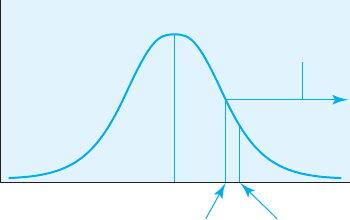
FIGURE 7.4
The t critical value
and the t obtained
for the single-
sample one-tailed
t test example
+2.06
Region
of rejection
+1.833
t
obt
t
cv
Interpreting the One-Tailed t Test
Our sample mean falls 2.06 standard deviations above the population mean
of 1090. We must now determine whether this is far enough away from the
population mean to be considered significantly different. In other words, is
our sample mean far enough away from the population mean that it lies in the
region of rejection? Because the alternative hypothesis is one-tailed, the region
of rejection is in only one tail of the sampling distribution. Consulting Table A.3
(in Appendix A) for a one-tailed test with alpha .05 and df N 1 9, we
see that t
cv
1.833. The t
obt
of 2.06 is therefore within the region of rejection. We
reject H
0
and support H
a
. In other words, we have sufficient evidence to allow
us to conclude that biology majors have significantly higher SAT scores than
the rest of the students at General University. Figure 7.4 illustrates the obtained
t in relation to the region of rejection. In APA style, the result is reported as
t(9) 2.06, p .05 (one-tailed)
This form conveys in a concise manner the t-score, the degrees of freedom,
that the results are significant at the .05 level, and that a one-tailed test was
used.
Calculations for the Two-Tailed t Test
What if the biology department made no directional prediction concerning
the SAT scores of its students? In other words, suppose the members of the
department are unsure whether their students’ SAT scores are higher or
lower than those of the general population of students and are simply inter-
ested in whether biology students differ from the population. In this case,
the test of the alternative hypothesis is two-tailed, and the null and alterna-
tive hypotheses are
H
0
:
0
1
, or
biology students
=
general population
H
a
:
0
1
, or
biology students
general population
10017_07_ch7_p163-201.indd 187 2/1/08 1:24:57 PM
188
■ ■
CHAPTER 7
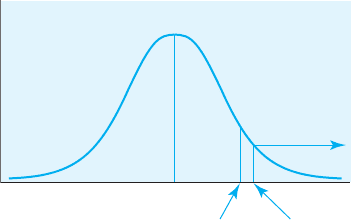
FIGURE 7.5
The t critical value
and the t obtained
for the single-
sample two-tailed t
test example
+2.262+2.06
t
cv
t
obt
If we assume that the sample of biology students is the same, then
X ,
s, and s
X
are all the same. The population at General University is also the
same, so is still 1090. Using all of this information to conduct the t test,
we end up with exactly the same t-test score of ±2.06. What, then, is the dif-
ference for the two-tailed t test? It is the same as the difference between the
one- and two-tailed z tests—the critical values differ.
Interpreting the Two-Tailed t Test
Remember that with a two-tailed alternative hypothesis, the region
of rejection is divided evenly between the two tails (the positive and
negative ends) of the sampling distribution. Consulting Table A.3 for a
two-tailed test with alpha .05 and df N – 1 9, we see that t
cv
2.262.
The t
obt
of 2.06 is therefore not within the region of rejection. We do not
reject H
0
and thus cannot support H
a
. In other words, we do not have suf-
ficient evidence to allow us to conclude that the population of biology
majors differs significantly on SAT scores from the rest of the students at
General University. Thus, with exactly the same data, we rejected H
0
with
a one-tailed test but failed to reject H
0
with a two-tailed test, illustrating
once again that one-tailed tests are more powerful than two-tailed tests.
Figure 7.5 illustrates the obtained t for the two-tailed test in relation to the
region of rejection.
Assumptions and Appropriate Use
of the Single-Sample t Test
The t test is a parametric test, as is the z test. As a parametric test, the
t test must meet certain assumptions. These assumptions include that the
data are interval or ratio and that the population distribution of scores is
symmetrical. The t test is used in situations that meet these assumptions
and in which the population mean is known, but the population standard
deviation () is not known. In cases where these criteria are not met,
a nonparametric test such as a chi-square test or Wilcoxon test is more
appropriate.
10017_07_ch7_p163-201.indd 188 2/1/08 1:24:58 PM

Hypothesis Testing and Inferential Statistics
■ ■
189
Confidence Intervals based
on the t Distribution
You might remember from our previous discussion of confidence intervals
that they allow us to estimate population means based on sample data (a
sample mean). Thus, when using confidence intervals, rather than deter-
mining whether the sample mean differs significantly from the population
mean, we are estimating the population mean based on knowing the sample
mean. We can use confidence intervals with the t distribution just as we did
with the z distribution (the area under the normal curve).
The t Test IN REVIEW
CONCEPT DESCRIPTION USE/EXAMPLE
Estimated standard The estimated standard deviation of a sampling Used in the calculation of
error of the mean ( s
X
) distribution, calculated by dividing s by
__
N a t test
t test Indicator of the number of standard deviation An inferential statistical
units the sample mean is from the mean of the test that differs from the
sampling distribution z test in that the sample size
is small (usually 30) and
is not known
One-tailed t test A directional inferential test in which a prediction H
a
:
0
1
is made that the population represented by the sample or
will be either above or below the general population H
a
:
0
1
Two-tailed t test A nondirectional inferential test in which the H
a
:
0
1
prediction is made that the population represented
by the sample will differ from the general population,
but the direction of the difference is not predicted
CRITICAL
THINKING
CHECK
7.5
1. Explain the difference in use and computation between the z test
and the t test.
2. Test the following hypothesis using the t test: Researchers are
interested in whether the pulses of long-distance runners dif-
fer from those of other athletes. They suspect that the runners’
pulses will be slower. They obtain a random sample (N 8) of
long-distance runners, measure their resting pulses, and obtain
the following data: 45, 42, 64, 54, 58, 49, 47, 55 beats per minute.
The average resting pulse of athletes in the general population is
60 beats per minute.
10017_07_ch7_p163-201.indd 189 2/1/08 1:24:58 PM
190
■ ■
CHAPTER 7
Let’s use the previous example in which we know the sample mean SAT
score for the biology students (
X 1176), the estimated standard error of
the mean ( s
X
41.71), and the sample size (N 10). We can calculate a con-
fidence interval based on knowing the sample mean and s
X
. Remember that
a confidence interval is an interval of a certain width, which we feel “confi-
dent” will contain . We are going to calculate a 95% confidence interval—in
other words, an interval that we feel 95% confident contains the population
mean. To calculate a 95% confidence interval using the t distribution, we
use Table A.3 “Critical Values for the Student’s t Distribution” (in Appendix
A) to determine the critical value of t at the .05 level. We use the .05 level
because 1 minus alpha tells us how confident we are, and, in this case, 1
is 1 .05 95%.
For a one-sample t test, the confidence interval is determined with the
following formula:
X ± t
cv
s
X
We already know
X (1176) and s
X
(41.71), so all we have left to determine is
t
cv
. We use Table A.3 to determine the t
cv
for the .05 level and a two-tailed test.
We always use the t
cv
for a two-tailed test because we are describing values
both above and below the mean of the distribution. Using Table A.3, we find
that the t
cv
for 9 degrees of freedom (remember df N – 1) is 2.262. We now
have all of the values we need to determine the confidence interval.
Let’s begin by calculating the lower limit of the confidence interval:
1176 2.262(41.71)
1176 94.35 1081.65
The upper limit of the confidence interval is
1176 2.262(41.71)
1176 94.35 1270.35
Thus, we can conclude that we are 95% confident that the interval of SAT
scores from 1081.65 to 1270.35 contains the population mean ().
As with the z distribution, we can calculate confidence intervals for the
t distribution that give us greater or less confidence (for example, a 99%
confidence interval or a 90% confidence interval). Typically, statisticians
recommend using either the 95% or 99% confidence interval (the intervals
corresponding to the .05 and .01 alpha levels in hypothesis testing). You have
likely encountered such intervals in real life. They are usually phrased in
terms of “plus or minus” some amount called the margin of error. For exam-
ple, when a newspaper reports that a sample survey showed that 53% of the
viewers support a particular candidate, the margin or error is typically also
reported—for example, “with a ±3% margin of error.” This means that the
researcher who conducted the survey created a confidence interval around
the 53% and that if they actually surveyed the entire population, would be
within ±3% of the 53%. In other words, they believe that between 50% and
56% of the viewers support this particular candidate.
10017_07_ch7_p163-201.indd 190 2/1/08 1:24:58 PM

Hypothesis Testing and Inferential Statistics
■ ■
191
The Chi-Square (
2
) Goodness-of-Fit Test:
What It Is and What It Does
The chi-square (
2
) goodness-of-fit test is a nonparametric statistical test
used for comparing categorical information against what we would expect
based on previous knowledge. As such, it tests the observed frequency (the
frequency with which participants fall into a category) against the expected
frequency (the frequency expected in a category if the sample data repre-
sent the population). It is a nondirectional test, meaning that the alternative
hypothesis is neither one-tailed nor two-tailed. The alternative hypothesis
for a
2
goodness-of-fit test is that the observed data do not fit the expected
frequencies for the population, and the null hypothesis is that they do fit
the expected frequencies for the population. There is no conventional way
to write these hypotheses in symbols, as we have done with the previous
statistical tests. To illustrate the
2
goodness-of-fit test, let’s look at a situation
in which its use is appropriate.
Calculations for the
2
Goodness-of-Fit Test
Suppose that a researcher is interested in determining whether the teen-
age pregnancy rate at a particular high school is different from the rate
statewide. Assume that the rate statewide is 17%. A random sample
of 80 female students is selected from the target high school. Seven of
the students are either pregnant now or have been pregnant previously.
The
2
goodness-of-fit test measures the observed frequencies against the
expected frequencies. The observed and expected frequencies are pre-
sented in Table 7.3.
As shown in the table, the observed frequencies represent the number
of high school females in the sample of 80 who were pregnant versus not
pregnant. The expected frequencies represent what we would expect based
on chance, given what is known about the population. In this case, we
would expect 17% of the females to be pregnant because this is the rate
statewide. If we take 17% of 80 (0.17 80 14), we would expect 14 of
the students to be pregnant. By the same token, we would expect 83% of
the students (0.83 80 66) to be not pregnant. If the calculated expected
frequencies are correct, when summed, they should equal the sample size
(14 66 80).
chi-square (
2
) goodness-
of-fit test A nonparametric
inferential procedure that de-
termines how well an observed
frequency distribution fits an
expected distribution.
chi-square (
2
) goodness-
of-fit test A nonparametric
inferential procedure that de-
termines how well an observed
frequency distribution fits an
expected distribution.
observed frequency
The frequency with which
participants fall into a category.
observed frequency
The frequency with which
participants fall into a category.
expected frequency
The frequency expected in a
category if the sample data
represent the population.
expected frequency
The frequency expected in a
category if the sample data
represent the population.
TABLE 7.3 Observed and Expected Frequencies for the
2
Goodness-of-Fit Example
FREQUENCIES PREGNANT NOT PREGNANT
Observed 7 73
Expected 14 66
10017_07_ch7_p163-201.indd 191 2/1/08 1:24:59 PM