Jean-Laurent Mallet. Geomodeling
Подождите немного. Документ загружается.

138
In
practice,
the
choice
of a
tessellation method depends
not
only
on the
nature
of
the
data
controlling
the
geometry
of the
object
to be
modeled,
but
also
on
the
usage
of the
model itself.
For
example
•
Structural
geologists
have
to
build
surfaces
defined
by
series
of
cross
sections.
In
this case, patch, strip,
and
pants algorithms
will
probably
be
their
preferred
tools.
•
Reservoir
engineers
are
primarily
interested
in
building
regular
and
irregular
3-grids
to be
used
as
geometrical support
by finite
elements methods.
It
should
be
noted
that
the
goal
of the
tessellation methods presented
in
this
chapter
is
only
to
give
a first-draft
discrete model
that
will
next
be
refined
and
modified
to
honor
all the
data
currently available.
It
will
be
demonstrated
in
the
next chapter,
as
well
as in
chapter
6,
that
the
DSI
method
is
particularly
well
adapted
to
this purpose.
CHAPTER 3. TESSELLATION
Chapter
4
Discrete Smooth
Interpolation=
This chapter presents
in
full
the
mathematical aspects
of
the
Discrete
Smooth
Interpolation method
(DSI)
introduced
in
chapter
1.
4.1
Introduction
4.1.1
Notations
Let us
consider
a
discrete model
J\A
n
(£l,
AT,
<£>,
C]
where
(p(o)
is
assumed
to be
a
vectorial
function
with
n
components
denned
on
J7:
The
set
0
is
assumed
to
contain
|0|
= M
nodes (see page
5)
so
that
the set of
values
{^"(a)
: a €
0,
v
=
1,...,
n}
contains
(n • M)
elements,
which
are
dispatched
as
follows
into
n
column matrices
j^
: v
=
1,..
.,n}
of the
same size
M and
into
one
global column
matrix
(p
of
size
139
140
CHAPTER
4.
DISCRETE SMOOTH INTERPOLATION
From
a
practical point
of
view,
in the following
pages,
no
distinction
will
be
made between
• the
function
<p"(-)
and its
associated
column vector
(f
v
of
size
M
• the
function
</?(•)
and its
associated
column vector
(p
of
size
(n • M)
The
soft
and
hard constraints
c € C
defined
by
equations
(1.4),
(1.5),
and
(1.6)
have
the
following
general "canonic"
form
where
M
stands
for one of the
following
operators:
In
this chapter,
we
will
assume
that
the (n • M)
coefficients
{A"(a}
:
a E
£7,
v =
1,...,
n}
have been gathered into
a
column matrix
A
c
of
size
(n •
M),
similar
to
(p
in
equation
(4.2),
in
such
a way
that
we can
write
It
should
be
noted
that
both members
of the
above equation
can be
divided
by
a
strictly positive constant without modifying
the
associated
constraint.
This
is the
reason
why the
assumption
has
been made throughout this book
that
each
constraint
c G
C~
has
been
"normalized"
in
such
a way
that
the
Euclidean
norm
of
A
c
is
equal
to
1:
The
most simple constraint corresponds
to the
notion
of
Control-Node
or
"fuzzy"
Control-Node
i
G fi
where
</?(£)
must
be
equal
to a
given value
(j)f.
Such
a
constraint
c =
c(£,
0^)
belongs
to
C
=
in the
case
of a
Control-Node
or
C~
in the
case
of a
"fuzzy"
Control-Node
and is
associated
with
the
following
coefficients:
4.1.
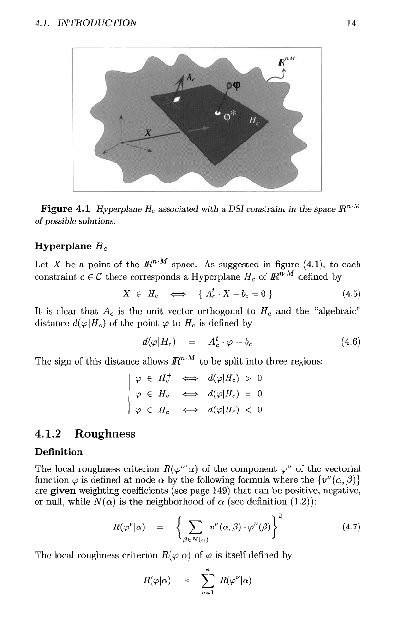
Figure
4.1
Hyperplane
H
c
associated
with
a
DSI
constraint
in the
space
JR
n
'
M
of
possible
solutions.
Hyperplane
H
c
Let X be a
point
of the
IR
n
'
space.
As
suggested
in
figure
(4.1),
to
each
constraint
c £ C
there corresponds
a
Hyperplane
H
c
of
lR
n
defined
by
It is
clear
that
A
c
is the
unit vector orthogonal
to
H
c
and the
"algebraic"
distance
d((p\H
c
)
of the
point
</?
to
H
c
is
defined
by
The
sign
of
this
distance allows
]R
n
to be
split
into
three
regions:
4.1.2 Roughness
Definitio n
The
local roughness criterion
R((p"\oi)
of the
component
<p
v
of the
vectorial
function
(f>
is
defined
at
node
a by the
following
formula
where
the
{v
v
(a,
(3}}
are
given
weighting
coefficients
(see page 149)
that
can be
positive, negative,
or
null,
while
N(a)
is the
neighborhood
of a
(see
definition
(1.2)):
The
local roughness criterion
R((p\a)
of
(p
is
itself
defined
by
INTRODUCTION
141
142
CHAPTER
4.
DISCRETE SMOOTH I
NTERPOLATION
R((f\a)
is
then
used
to
build
a
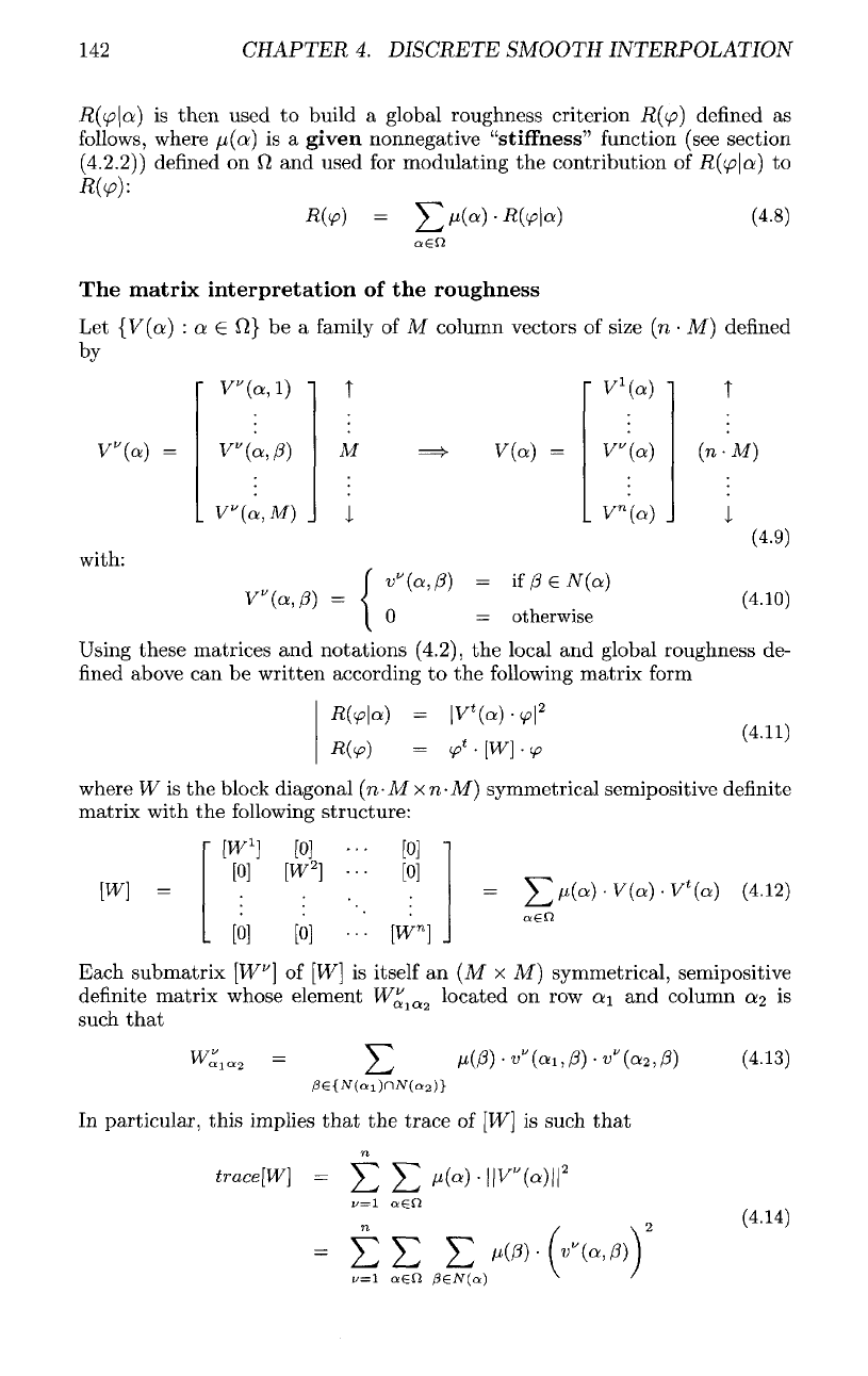
global roughness criterion
R(tp)
denned
as
follows,
where
n(ot)
is a
given
nonnegative
"stiffness"
function (see
section
(4.2.2))
defined
on
0
and
used
for
modulating
the
contribution
of
R((f>\a)
to
R(vY
The
matrix
interpretation
of the
roughness
Let
(V(ct)
: a
e
Q}
be a
family
of M
column vectors
of
size
(n • M)
defined
by
Using
these matrices
and
notations
(4.2),
the
local
and
global roughness
de-
nned
above
can be
written according
to the
following
matrix
form
where
W is the
block
diagonal
(n-M
x
n-M]
symmetrical
semipositive definite
matrix with
the
following
structure:
Each submatrix
\W
V
]
of [W] is
itself
an (M x M)
symmetrical, semipositive
definite
matrix whose element
W£
ia2
located
on row
a\
and
column
a
2
is
such
that
In
particular,
this
implies
that
the
trace
of
[W]
is
such
that
4.1.
INTRODUCTI
ON
Commen t
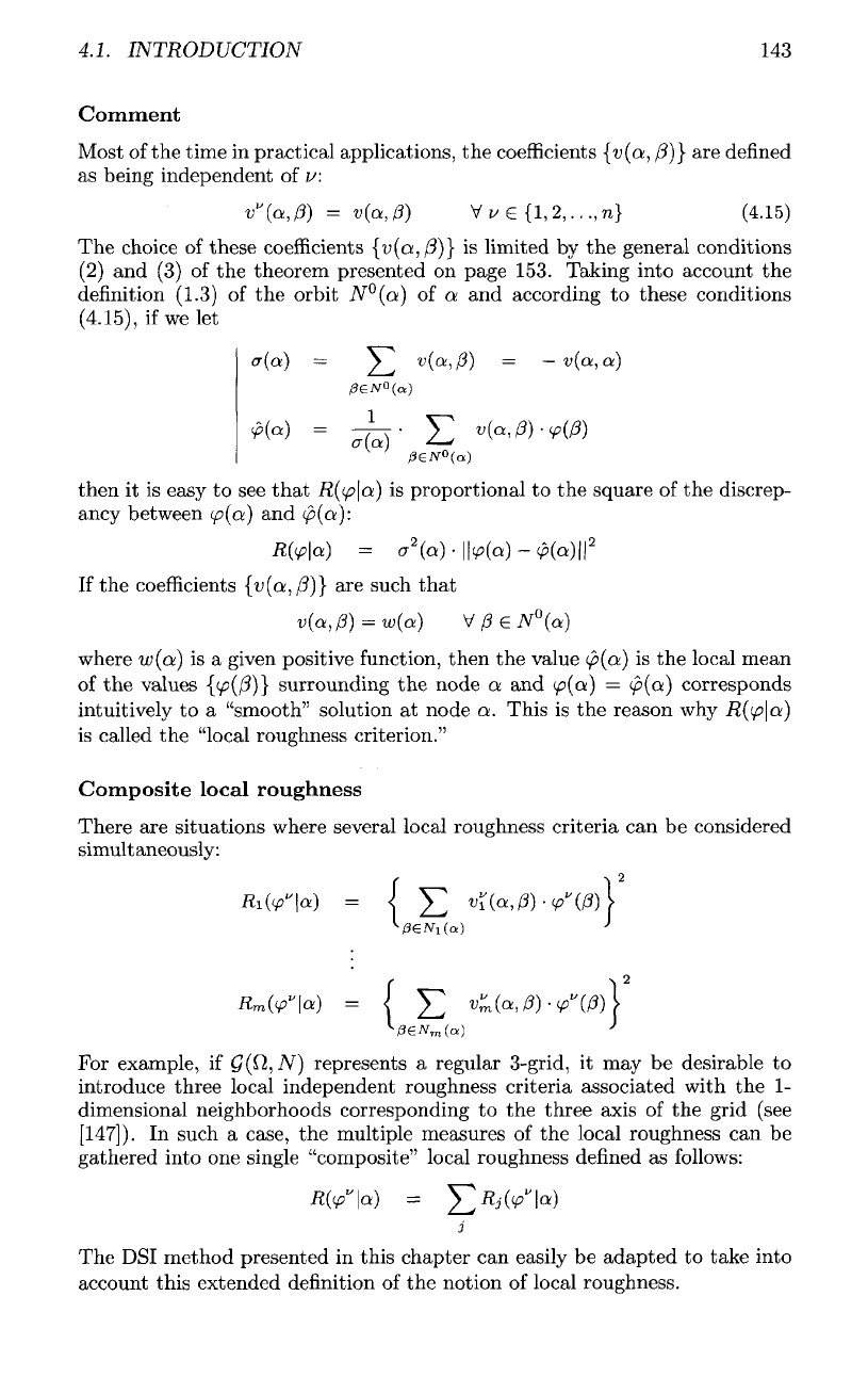
Most
of the
time
in
practical applications,
the
coefficients
{v(a,
(3)}
are
defined
as
being independent
of
v:
The
choice
of
these
coefficients
{v(a,(3}}
is
limited
by the
general conditions
(2)
and (3) of the
theorem presented
on
page
153.
Taking into account
the
definition
(1.3)
of the
orbit
N°(a)
of a and
according
to
these conditions
(4.15),
if
we let
then
it is
easy
to see
that
R((p\a)
is
proportional
to the
square
of the
discrep-
ancy between
(p(a)
and
<p(ct):
If
the
coefficients
{i>(a,
/?)}
are
such
that
where
w(a)
is a
given positive
function,
then
the
value
<p(a)
is the
local mean
of
the
values
{</?(/?)}
surrounding
the
node
a and
(p(a)
=
<p(ot)
corresponds
intuitively
to a
"smooth" solution
at
node
a.
This
is the
reason
why
R((p\a)
is
called
the
"local roughness criterion."
Composite local roughness
There
are
situations where several local roughness criteria
can be
considered
simult
aneously:
For
example,
if
Q(£t,
N]
represents
a
regular 3-grid,
it may be
desirable
to
introduce
three local independent roughness criteria associated with
the 1-
dimensional
neighborhoods corresponding
to the
three axis
of the
grid
(see
[147]).
In
such
a
case,
the
multiple measures
of the
local roughness
can be
gathered into
one
single "composite" local roughness
defined
as
follows:
The
DSI
method presented
in
this chapter
can
easily
be
adapted
to
take into
account
this
extended definition
of the
notion
of
local roughness.
14.3
144
CHAPTER
4.
DISCRETE SMOOTH INTERPOLATION
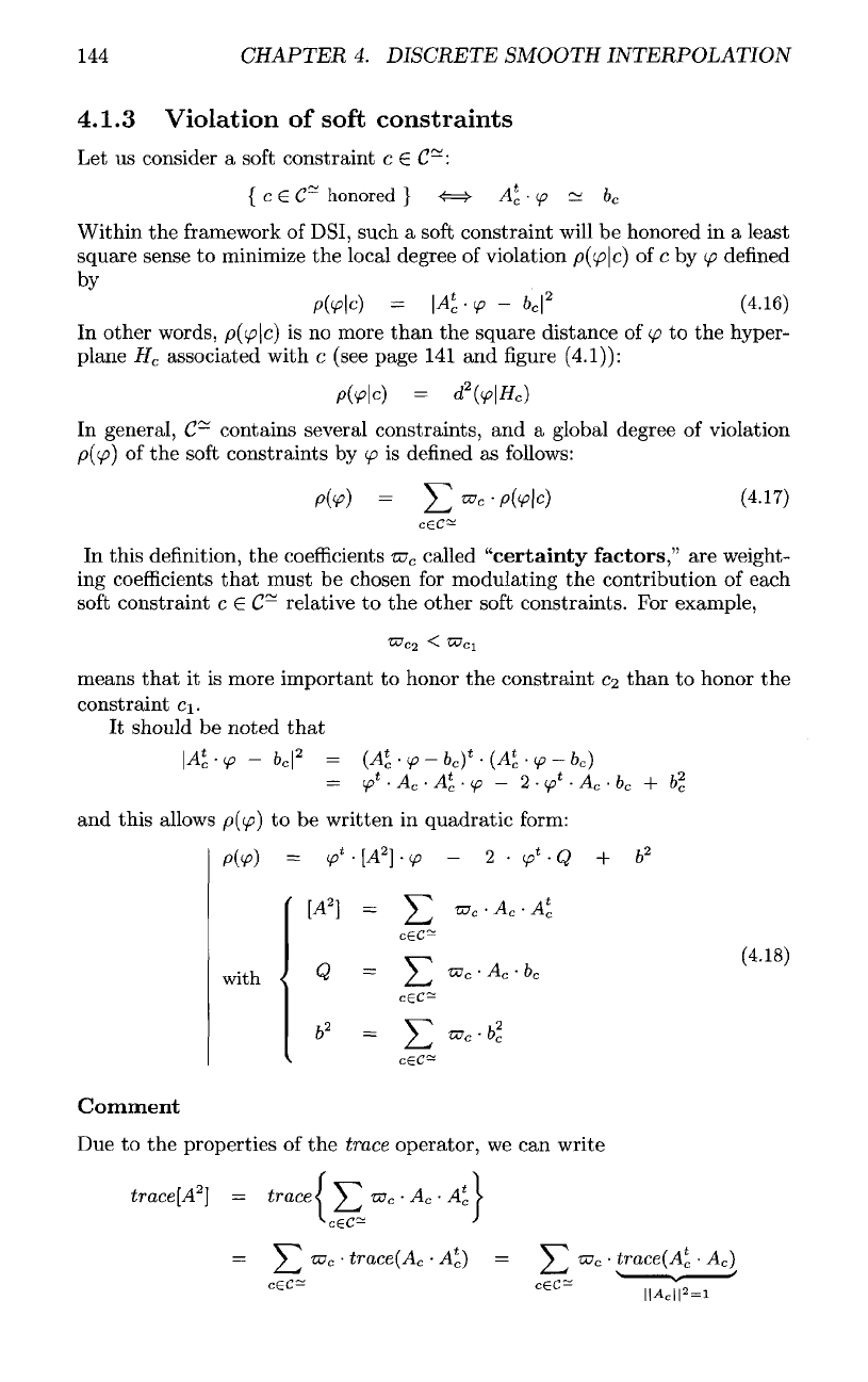
4.1.3
Violation
of
soft
constraints
Let us
consider
a
soft
constraint
c G
C~:
Within
the
framework
of
DSI,
such
a
soft
constraint
will
be
honored
in a
least
square sense
to
minimize
the
local degree
of
violation
p((/?|c)
of c by
</?
defined
by
In
other
words,
p((p\c}
is no
more
than
the
square distance
of
<p
to the
hyper-
plane
H
c
associated with
c
(see page
141 and
figure
(4.1)):
In
general,
C~
contains several constraints,
and a
global degree
of
violation
p((p)
of the
soft
constraints
by
(p
is
denned
as
follows:
In
this
definition,
the
coefficients
w
c
called
"certainty
factors,"
are
weight-
ing
coefficients
that
must
be
chosen
for
modulating
the
contribution
of
each
soft
constraint
c 6
C~
relative
to the
other
soft
constraints.
For
example,
means
that
it is
more important
to
honor
the
constraint
02
than
to
honor
the
constraint
c\.
It
should
be
noted
that
and
this allows
p((p)
to be
written
in
quadratic
form:
Comment
Due
to the
properties
of the
trace
operator,
we can
write
4.1.
INTRODUCTION
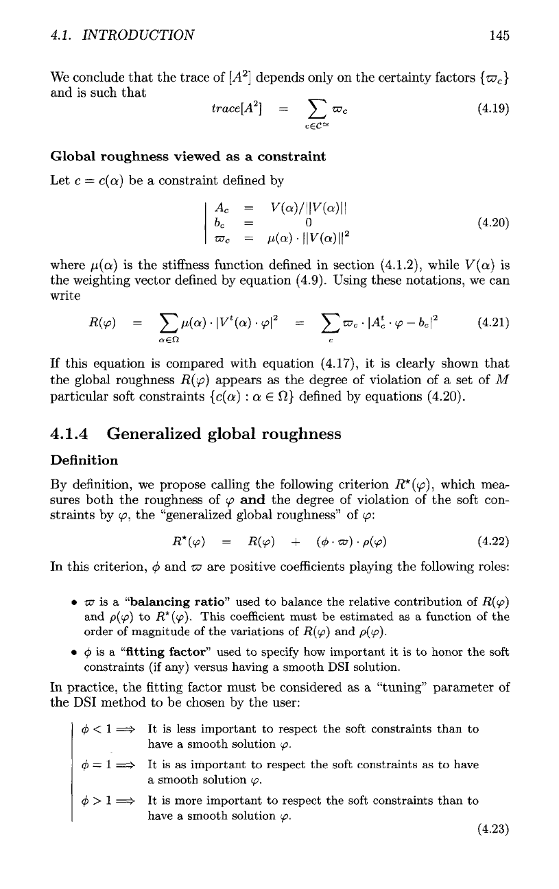
We
conclude
that
the
trace
of
[A
2
]
depends only
on the
certainty factors
{w
c
}
and is
such
that
Global
roughness
viewed
as a
constraint
Let
c =
c(a)
be a
constraint
defined
by
where
//(a)
is the
stiffness function defined
in
section (4.1.2), while
V(a)
is
the
weighting vector
defined
by
equation
(4.9).
Using these notations,
we can
write
If
this equation
is
compared with equation (4.17),
it is
clearly shown
that
the
global roughness
R((f>}
appears
as the
degree
of
violation
of a set of
M
particular
soft
constraints
{c(a)
:
a 6 0}
defined
by
equations
(4.20).
4.1.4 Generalized global roughness
Definition
By
definition,
we
propose calling
the
following
criterion
R*(<p],
which mea-
sures both
the
roughness
of
(p
and the
degree
of
violation
of the
soft
con-
straints
by
(/?,
the
"generalized global roughness"
of
<p:
In
this criterion,
0 and
w
are
positive
coefficients
playing
the
following
roles:
•
w
is a
"balancing ratio"
used
to
balance
the
relative
contribution
of
R((p)
and
p(np)
to
/?*(</?).
This
coefficient
must
be
estimated
as a
function
of the
order
of
magnitude
of the
variations
of
R(<p}
and
p(<p).
•
(p
is a
"fitting factor" used
to
specify
how
important
it is to
honor
the
soft
constraints
(if
any)
versus
having
a
smooth
DSI
solution.
In
practice,
the fitting
factor must
be
considered
as a
"tuning"
parameter
of
the DSI
method
to be
chosen
by the
user:
0
< 1
=>
It is
less
important
to
respect
the
soft
constraints than
to
have
a
smooth
solution
<p.
0=1
=>•
It is as
important
to
respect
the
soft
constraints
as to
have
a
smooth
solution
(p.
(f)
>
I
==>
It is
more
important
to
respect
the
soft
constraints than
to
have
a
smooth
solution
(p.
145
This implies
that
the
balancing ratio
w
must
be
chosen according
to the
following
equation:
From equations
(4.14),
and
(4.19),
we
conclude
that
w
should
be
chosen
as
follows:
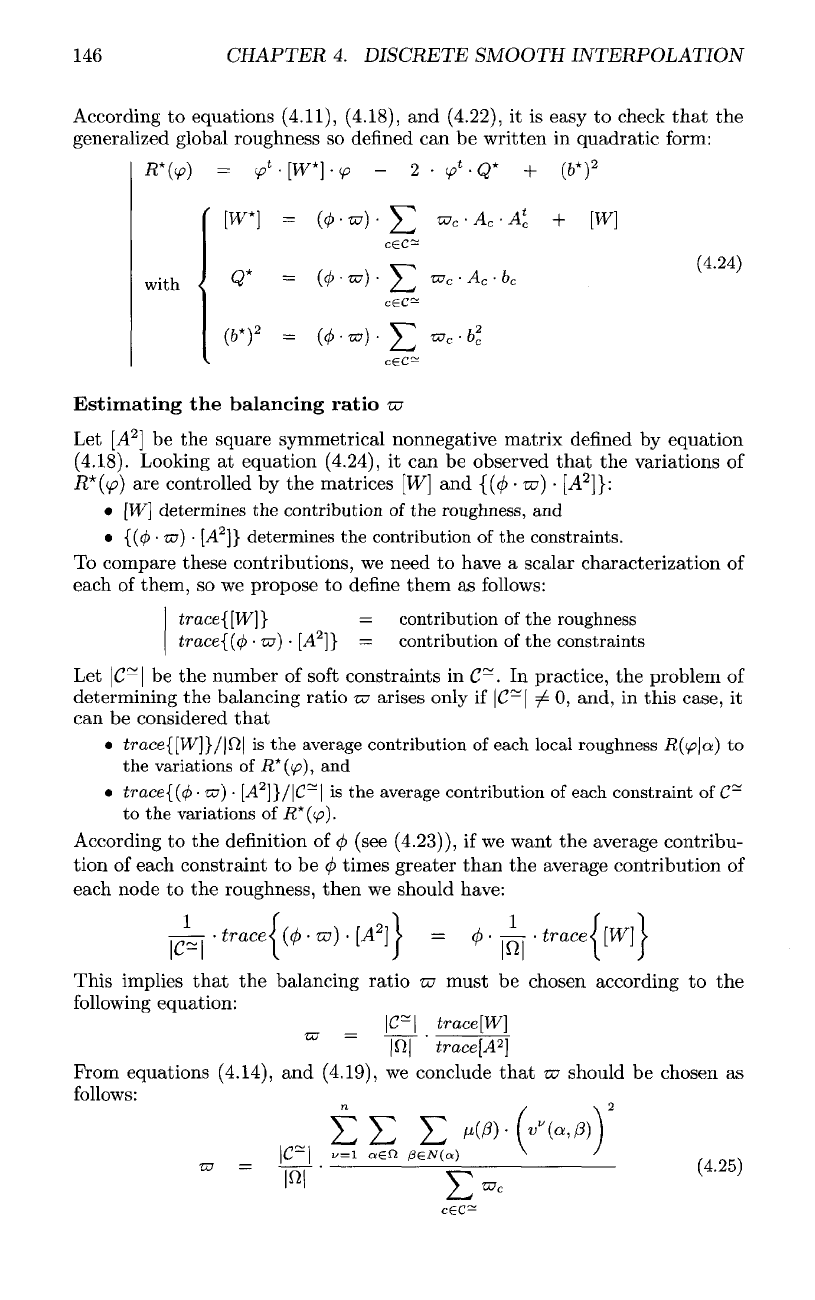
According
to
equations (4.11),
(4.18),
and
(4.22),
it is
easy
to
check
that
the
generalized global roughness
so
defined
can be
written
in
quadratic
form:
Estimating
the
balancing
ratio
w
Let
[A
2
]
be the
square symmetrical nonnegative matrix
denned
by
equation
(4.18).
Looking
at
equation
(4.24),
it can be
observed
that
the
variations
of
R*(tp]
are
controlled
by the
matrices
[W] and
{(</>•
-a?)
•
[A
2
]}:
•
[W]
determines
the
contribution
of the
roughness,
and
•
{(0
•
ru)
•
[A
2
]}
determines
the
contribution
of the
constraints.
To
compare these
contributions,
we
need
to
have
a
scalar characterization
of
each
of
them,
so we
propose
to
define
them
as
follows:
trace{[W]}
=
contribution
of the
roughness
trace{((f)
• w) •
[A
2
]}
—
contribution
of the
constraints
Let
C~\
be the
number
of
soft
constraints
in
C~.
In
practice,
the
problem
of
determining
the
balancing ratio
TU
arises only
if
\C~\
^
0,
and,
in
this
case,
it
can
be
considered
that
•
trace{[W]}/|fi|
is the
average contribution
of
each local roughness
R((p\Oi)
to
the
variations
of
R*(tf>),
and
•
trace{((/>
•
w}
•
[A
2
]}/\C~
is the
average contribution
of
each constraint
of
C~
to the
variations
of
R*(yy).
According
to the
definition
of
0
(see
(4.23)),
if we
want
the
average contribu-
tion
of
each
constraint
to be
0
times
greater
than
the
average
contribution
of
each node
to the
roughness, then
we
should have:
146
CHAPTER 4. DISCRETE SMOOTH INTERPOLATION
4.2.
THE
DSI
PROBLEM
147
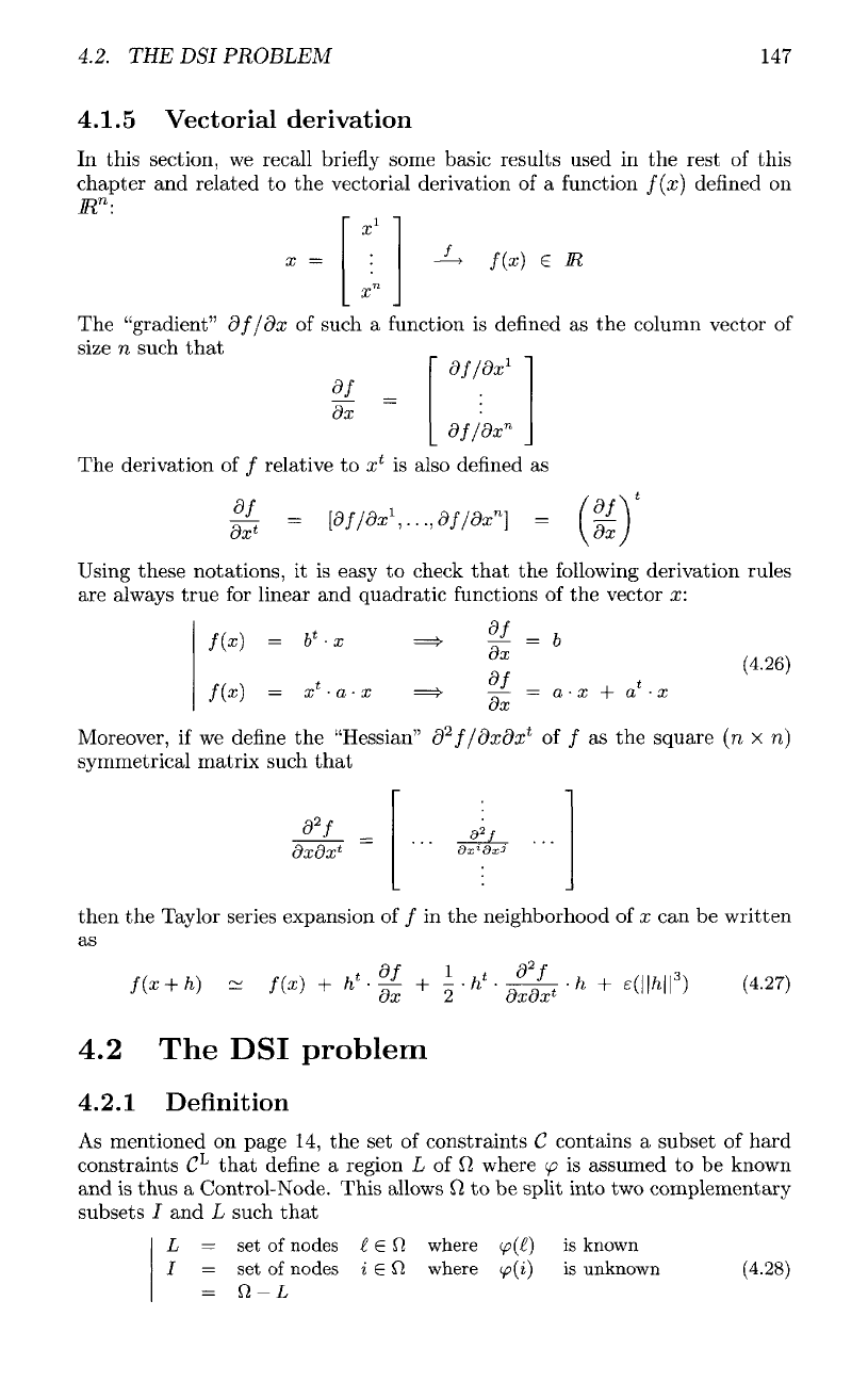
4.1.5 Vectorial
derivation
In
this section,
we
recall
briefly
some basic results used
in the
rest
of
this
chapter
and
related
to the
vectorial derivation
of a
function
f(x)
denned
on
M
n
:
Using
these
notations,
it is
easy
to
check
that
the
following
derivation rules
are
always true
for
linear
and
quadratic
functions
of the
vector
x:
Moreover,
if we
define
the
"Hessian"
d
2
f/dxdx
t
of / as the
square
(n
x
n)
symmetrical matrix such
that
then
the
Taylor series expansion
of / in the
neighborhood
of x can be
written
as
4.2
The DSI
problem
4.2.1 Definition
As
mentioned
on
page
14, the set of
constraints
C
contains
a
subset
of
hard
constraints
C
L
that
define
a
region
L
of 0
where
(p
is
assumed
to be
known
and is
thus
a
Control-Node.
This
allows
Q
to be
split into
two
complementary
subsets
/ and
L
such
that
L = set of
nodes
t
G
^
where
<£>(£)
is
known
/ = set of
nodes
i G fi
where
<p(i)
is
unknown
=
n-L
The
"gradient"
df/dx
of
such
a
function
is
defined
as the
column vector
of
size
n
such
that
The
derivation
of /
relative
to
x*
is
also
defined
as