Korn G.A. Advanced Dynamic-system Simulation: Model-replication Techniques and Monte Carlo Simulation
Подождите немного. Документ загружается.

92 Parameter-influence Studies, Model Replication, and Monte Carlo Simulation
with
v = sqrt(xdot
2
+ ydot
2
)
The acceleration due to gravity g = 32.2 ft/s
2
and R = 7.5E-05 ft
–1
is the drag
coefficient divided by the projectile mass. The trajectory of each shot is then
determined by the initial muzzle position
x(0) = y(0) = 0 and the initial veloc-
ity components
xdot(0) = v0 * cos(theta0) ydot(0) = v0 * sin(theta0) (4-10)
theta0 is the gun elevation angle, and v0 = 900 ft/s is the given muzzle velocity.
Assuming level ground, the impact abscissa
xI is the value of x where y = 0
at the end of a trajectory. A good way to read
xI is with the track-hold differ-
ence equation
xI = xI + swtch(y) * (x - xI)
(Section 2-16b), which causes xI to track x while and then holds the x
value. The initial value of the difference-equation state variable xI defaults to 0.
To aim the cannon, we set the elevation angle
theta0 to obtain a desired
impact abscissa
xI, say theta0 = 70 * PI/180. Our Monte Carlo study then
adds random perturbations to this nominal gun elevation and determines their
effect on the sample average and sample variance of the impact coordinate
xI.
To get approximately Gaussian-distributed elevation errors, we set
theta0 = 70 * PI/180 + a * (ran()+ran()+ran()+ran())
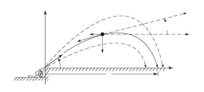
y
ϑ(O)
Instantaneous
direction of flight
mg
W(t)
D(v)
v(O)
Horizontal
X
X
I
ϑ
FIGURE 4-2. Cannon geometry (based on Reference [6]). We assume that the wind force
W(t) is zero.
Since ran() is uniformly distributed between –1 and 1 with expected value
0 and theoretical variance 1/3, we have
E{theta0} = 70 PI/180 Var{theta0} = 4 * a
2
/3
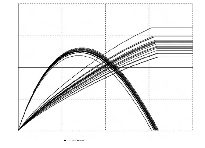
Figure 4-3 shows time histories of x(t) and the track-hold output xI(t) for a
few simulation runs together with the complete program for the repeated-run
Monte Carlo study. The program also displays the resulting sample average
xavg and the sample statistical dispersion s = sqrt(abs(xxavg – xavg^2)) of
the impact abscissa
xI after n runs.
4-7. Vectorized (Model-replicating) Monte Carlo Simulation
(a) Vectorized Monte Carlo Study of the 1776 Cannon Shot
Model-replicating or vectorized Monte Carlo simulation was originally
developed for supercomputer studies of small physics models, where the
repeated-run program overhead is especially significant. As we saw in
Section 4-2b, our vector compiler conveniently implements vectorization on
inexpensive personal computers, where its advantages—simpler programs
and high speed, at least for small models—are welcome indeed. As an added
bonus, vectorization can also help check the quality of pseudorandom noise
(Section 5-10).
Instead of repeating simulated cannon shots as in Section 4-6, the experiment
protocol in Figure 4-4 declares
n-dimensional state-variable and arrays (vectors)
STATE x[n], y[n], xdot[n], ydot[n] | ARRAY theta0[n], v[n], xImpact[n]
and loops to “fill” each of the arrays theta0, xdot, and ydot with n different
random initial values:
for i = 1 to n | -- noisy elevation angle in radians
theta0[i] = 70 * PI/180 + a * (ran()+ran()+ran()+ran())
xdot[i] = v0 * cos(theta0[i]) | ydot[i] = v0 * sin(theta0[i])
next
A vectorized DYNAMIC program segment then effectively replicates the
cannonball model and the output track/hold operation
n times:
Vector v = sqrt(xdot^2 + ydot^2) | -- a defined variable
Vectr d/dt x = xdot | Vectr d/dt y = ydot | -- equations of motion
Vectr d/dt xdot = - R * v * xdot | Vectr d/dt ydot = - R * v * ydot - g
--
step
Vector xImpact = xImpact + swtch(y) * (x - xImpact) | -- track-hold
Monte Carlo Simulation of Dynamic Systems 93
xl
+
0
–
025→ 50
scale = 5000 Y,XX vs. t
— REPEATED-RUN MONTE CARLO: 1776 CANNON
----------------------------------------------------------------------------------------------------
DT = 0.008 | TMAX = 50 | NN = 5000 | scale=5000
----------------------------------------------------------------------------------------------------
R = 7.5E-05 | g = 32.2
v0 = 900 | –– muzzle velocity
a = 0.03 | –– noise amplitude
––
n = 1000 | ARRAY xImpact[n] | –– sample values
––
for i = 1 to n | –– elevation in radians
xI = 0 | –– initialize track-hold
theta0 = 70 * PI/180 + a * (ran()+ran()+ran()+ran())
xdot = v0 * cos(theta0) | ydot = v0 * sin(theta0)
drunr | display 2 | –– run, don’t erase display
xImpact[i] = xI | –– read the impact abscissa xI
next
– – COMPUTE STATISTICS AFTER n RUNS
––
DOT xSum = xImpact * 1 | xAvg = xSum/n
DOT xxSum = xImpact * xImpact | xxAvg = xxSum/n
s = sqrt(abs(xxAvg - xAvg^2)) | – – dispersion
write “xAvg = “;xAvg,” s = “;s
--------------------------------------------
DYNAMIC
--------------------------------------------
v = sqrt(xdot^2 + ydot^2)
d/dt x = xdot | d/dt y = ydot
d/dt xdot = - R * v * xdot | d/dt ydot = - R * v * ydot-g
––
step
xI = xI + swtch(y) * (x - xI) | – – hold the impact abscissa
94

Monte Carlo Simulation of Dynamic Systems 95
Figure 4-4 shows the complete program. The vectorized cannonball study
produced essentially the same results as the repeated-run study, as
expected.
One thousand repeated runs and the statistics computation took 5 s on a
2.4-GHz Athlon64, and the equivalent vectorized study took 3.4 s. This
speed advantage is typical for small models. The repeated-run overhead
saved by vectorization becomes less significant as the model size
increases.
-- VECTORIZED MONTE CARLO STUDY: 1776 CANNON
----------------------------------------------------------------------------------------------------
DT = 0.008 | TMAX = 50 | NN = 5000 | scale=5000
R = 7.5E-05 | g = 32.2
v0 = 900 | -- muzzle velocity
a = 0.03 | -- noise amplitude
--
n = 1000 | STATE x[n], y[n], xdot[n], ydot[n]
ARRAY theta0[n], v[n], xImpact[n]
--
for i= 1 to n | -- noisy elevation angle in radians
theta0[i] = 70 * PI/180 + a * (ran()+ran()+ran()+ran())
xdot[i] = v0 * cos(theta0[i]) | ydot[i] = v0 * sin(theta0[i])
next
-- make a single simulation run …
drun | … and then compute statistics
--
DOT xSum = xImpact * 1 | xAvg = xSum/n
DOT xxSum = xImpact * xImpact | xxAvg = xxSum/n
s = sqrt(xxAvg - xAvg^2)
write “xAvg = “;xAvg,” s = “;s
----------------------------------------------------------------------------------------------------
DYNAMIC
----------------------------------------------------------------------------------------------------
Vector v = sqrt(xdot^2 + ydot^2)
Vectr d/dt x = xdot | Vectr d/dt y = ydot
Vectr d/dt xdot = - R * v * xdot | Vectr d/dt ydot = - R * v * ydot - g
--
step
Vector xImpact = xImpact + swtch(y) * (x - xImpact) | -- n track-holds
FIGURE 4-4. Complete program for a vectorized Monte Carlo study of the 1776 cannonball
problem. All initial
xImpact[i] default to 0.
FIGURE 4-3. This repeated-run Monte Carlo study determines the impact-range dispersion
of a 1776 cannon shot due to random elevation-setting errors. A track-hold difference equation
(Section 2-16b) holds the impact coordinate.
96 Parameter-influence Studies, Model Replication, and Monte Carlo Simulation
(b) Interactive Monte Carlo Simulation: Computing Time Histories of
Statistics with Compiled
DOT
Operations
Vectorized Monte Carlo simulation has another interesting and important
feature. Since a single simulation run samples all
n replicated models at each
point of time, one can compute and display time histories of statistics, and
observe the results of parameter changes as the simulation run proceeds.
Such interactive Monte Carlo simulation was formerly possible only with
very fast (and very inaccurate) analog computers [7].
Runtime statistics computations are needed only at output-sampling times,
not at every derivative call. We will thus save time by programming
DYNAMIC-segment statistics computations following an
OUT or SAMPLE
m statement (Section 1-6). As noted in Section 4-6a, most statistics are func-
tions of sample averages. A vectorized DYNAMIC program segment com-
putes the sample averages
qAvg(t) = (q[1] + q[2] + … + q[n])/n
qqAvg(t) = (q
2
[1] + q
2
[2] + … + q
2
[n])/n
of a replicated system variable q = q(t) at each sampling time t with
OUT
DOT qSum = q * 1 | qAvg = qSum/n
DOT qqSum = q * q | qqavg = qqSum/n
The value of 1/n can be precomputed by the experiment protocol to avoid
time-consuming divisions by
n. Unlike in Section 4-6, we are using compiled
DOT operations that, like DESIRE vector assignments, involve no program-
loop overhead (Section 3-7).
We could add runtime computation of
xAvg(t) and yAvg(t) to the vector-
ized cannonball study in Figure 4-4 and display the average trajectory (graph
of
yAvg(t) versus XAvg(t)). We shall exhibit more interesting applications in
Sections 5-8 and 5-9.
4-8. Statistical Relative Frequencies, Sample Ranges,
and Other Statistics
For any random variable
x in our Monte Carlo model, the sample statistical
relative frequency
hh of an event {a < x < b} (a < b) is the fraction of our n
process samples where a < x < b is true. hh estimates the probability of the
event. Instead of counting events, we measure
hh as the sample average
uAvg of the indicator function
u(x)
≡
swtch(x – a) – swtch(x – b) (a < b) (4-11)
Monte Carlo Simulation of Dynamic Systems 97
In the open class interval (a, b), u(x) = 1 and is 0 elsewhere (see also Section
2-8b). We find the desired statistical relative frequency
hh easily and quickly
with
DOT hh = u * 1.
Statistical relative frequencies can be computed as post-run Monte Carlo
statistics. Vectorized Monte Carlo studies can, instead, compute statistical
relative frequencies at each sampling point to produce their time histories.
For a given Monte Carlo sample
(x[1], x[2], …, x[n]), the sample range
range = xmax – xmin is the difference between the largest value xmax and
the smallest value
xmin in the sample. The DYNAMIC program segment of a
vectorized Monte Carlo study can compute
xmax, xmin, and range at each
point of time to produce their time histories. With reference to Section 3-8, we
declare an
n-dimensional vector xx and add the DYNAMIC-segment lines
Vector xx^ = x | DOT xmax = xx * 1
Vector xx^ = - x | DOT mxmin = xx * 1
The experiment-protocol script then computes range = xmax + mxmin.For
repeated-run Monte Carlo simulation, post-run computation of
xmax and
xmin requires a search loop in the experiment protocol.
As we already noted, many other statistics (correlation and regression
coefficients, and test statistics such as
t and χ
2
)[5] are functions of sample
averages. Post-run estimation of probability densities will be discussed in the
next section.
4-9. Post-run Probability-density Estimation [8,9]
(a) A Simple Probability-density Estimate
For continuous random variables x the probability density
ϕ
x
(X) for each
value
X of x is approximated by
ϕ
x
(X)
≈
Prob{X – h
<
–
x < X + h}/2h = p/2h
(4-12)
where
2h is a small class-interval width. For a given Monte Carlo sample
(x[1], x[2], ... , x[n]) of x-values, we again estimate p by the sample average
<u(x – X)> of an indicator function u(x – X) equal to 1 if X – h
<
–
x < X + h
and 0 otherwise. Specifically, u(x – X) ≡ rect((x – X)/h), where rect(x) is the
library function defined in Fig. 2-5c. For small “window widths”
2h we thus
estimate the probability density
ϕ
x
(X)
≈
p/2h by
f(X)
≡
(1/2h) <rect [(x – X)/h]
>
≡
(1/2hn)
n
k=1
rect ((x[k] – X)/h) (4-13)
98 Parameter-influence Studies, Model Replication, and Monte Carlo Simulation
For random samples of size n, 2hn f(X) has a binomial distribution with
success probability
p, [4] so that
E{f(X)} = p/2h, Var {f(X)} = p(1 – p)/4nh
2
(4-14)
and for small window widths
h
E{f(X)}
≈ ϕ
x
(X) Var {f(X)}
≈ ϕ
x
(X)[1 – 2h
ϕ
x
(X)]/2nh
≈ ϕ
x
(X)/2nh (4-15)
Because good resolution (small
h) implies fewer data points in each window
and thus larger estimate variances, probability-density measurement always
involves a compromise between resolution and variance. You may need a
large sample size
n.
(b) Triangle and Parzen Windows
[8,9]
We usually want to estimate
ϕ
x
(X) for multiple X-values and would like to fit
the estimated
ϕ
x
(X) values with a smooth curve. Estimates of
ϕ
x
(X) for dif-
ferent
X-values separated by less than the window width 2h effectively use
some sample values more than once. Qualitatively speaking, this means that
a curve fitted to the estimate points can be smoothed and appears to exhibit
less fluctuation than individual measurements would.
Improved probability-density estimates attempt to enhance this effect. We
replace the rectangle-window estimate (21) with the sample average
f(X)
≡
<k[(x – X)/h]/h> (4-16)
of a new bump-shaped kernel function
k[(x – X)/h]/h centered on the
argument
X of the desired estimate f(X). The window width h of a kernel
determines the spread of the bump and thus the resolution of the probability-
density estimate.
h can be made smaller for larger sample sizes n. Our prim-
itive rectangular window
rect[(x – X)/h]/2 “weights” all x-values falling into
its window equally and suppresses all others, but more general kernel func-
tions
k[(x – X)/h] let x-values farther away from the argument value X con-
tribute to the sample average. Since
ϕ
x
(X) is continuous, this provides a sort
of interpolation and may reduce the estimate variance for a given resolution.
The probability-density estimate
f(x) is correctly normalized if the kernel
function
k(X) is normalized, so that
⫺⬁
⬁
k(X) dX = 1 implies
⫺⬁
⬁
f(X) dX = 1
Monte Carlo Simulation of Dynamic Systems 99
The estimate mean and variance cannot be derived as easily as in Eq. (14).
But it can be shown [10] that
f(x) is an asymptotically unbiased and consis-
tent estimate of
ϕ
x
(X), and
Var{ f(X)}
→
(1/nh)
ϕ
x
(X) KK as n
→ ∞
with KK =
⫺
⬁
⬁
k
2
(q)dq (4-17)
provided that
⫺
⬁
⬁
k(X)
dx <
∞
, sup
(
−
⬁
,
⬁
)
k(X)
<
∞
lim
n
→
∞
[Xk(X)] = 0,
lim
n
→
∞
h(n) = 0 lim
n
→
∞
[nh(n)] =
∞
The rectangle-window estimate (13) is a special case of the estimate
(16); here
k(X)
≡
rect(X/h)/2 with KK = 1/2
The next-simplest example uses the triangle-window kernel
k(X)
≡
lim(1 – |X/h|) with KK = 2/3
In effect, this mixes x-values from three neighboring class intervals. But we
usually prefer the Parzen-window kernel
k(X)
≡
exp(–X
2
/2)/sqrt(2
π
) with KK = 1/[2sqrt(
π
)]
which gives some weight to all x-values. Its resolution-determining window
width
h measures the spread of a Gaussian-shaped kernel function.
(c) Computation and Display of Parzen Window Estimates
Given a post-run Monte Carlo sample (vector) x
≡
(x[1], x[2], …, x[n]), the
Parzen-window estimate of the probability density
ϕ
x
(X) is the average F(X)
of the n sample values
ff[i] = exp[– (X – x[i])
2
/2 h
2
] / [h * sqrt(2
π
)] (i = 1, 2, …, n) (4-18)
For each given sample size n, our choice of the window width h will be a
trial-and-error compromise between the
X resolution and the smoothness of
the estimated probability-density curve. To use smaller window widths
h, n
has to be increased.

100 Parameter-influence Studies, Model Replication, and Monte Carlo Simulation
For post-run estimation of probability densities, we add the lines
ARRAY f[n] | -- declare a vector of sample values f[i] = ff[i]/n
irule 0 | -- this DYNAMIC segment handles only sampled data
t = 0 | TMAX = 1
a = (select the range a = X2 – X1 of the X-sweep)
b = (select the starting value b = X1 of X)
NN = (select the number of estimated values)
h = (select the Parzen-window width)
alpha = 1/(2 * h^2) | beta = 1/(h * n * sqrt(2 * PI))
drun PARZEN
at the end of our experiment-protocol script, say of Figure 4-3 or 4-4. These
script lines set parameter values and then execute an extra DYNAMIC pro-
gram segment labeled
PARZEN, which will produce probability-density esti-
mates
F(X) for NN values of x between x = X1 and X = X2 as t increases from
t = 0 to t = TMAX = 1. Note that the values selected for NN, scale, and TMAX
are different from the values used for the simulation itself.
The extra DYNAMIC program segment computes and averages the expres-
sion (4-18) to produce
NN values of F(X) between X = t0 and X = t0 + TMAX:
label PARZEN
--
X = a * t + b | -- this sweeps X from X1 to X2 as t increases
-- compute n samples ff[i] = f[i]/n
Vector f = beta * exp(- alpha * (X - x)^2))
DOT F = f * 1 | -- sum to average (note that 1/n is included in beta)
dispxy X, F
Note that x is a vector of sample values, and X is a scalar. The last line plots
F(X) versus X. Since F is always positive, we usually display FF = c *
F – scale, where c is a scale factor. Figure 5-2c shows such a probability-
density display. The Parzen-window technique can be extended to multidi-
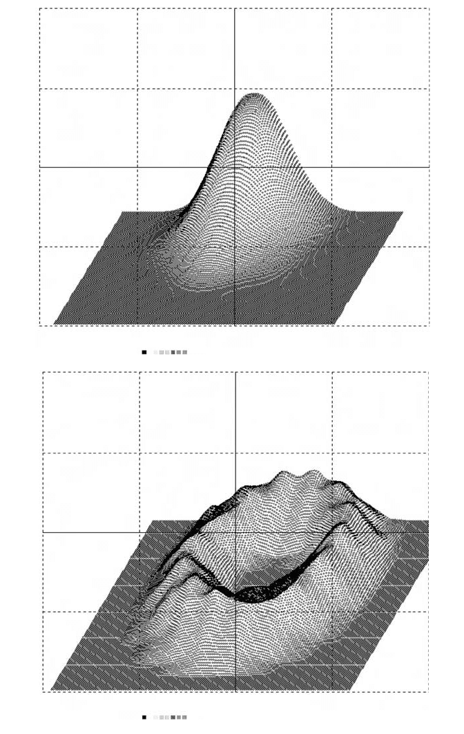
mensional probability distributions (Fig. 4-5).
4-10. Combining Vectorized and Repeated-run
Monte Carlo Simulation
Since model replication effectively multiplies the number of state variables
by
n, a simulation problem with many differential-equation state variables
may not fit a single vectorized Monte Carlo run.
6
6
Currently, DESIRE admits up to 40,000 (Linux) or 20,000 (Windows) differential-equation state
variables with Euler and fixed or variable-step Runge–Kutta integration (
irule 2–7), or up to 600
state variables with more advanced variable-step/variable-order integration (
irule 9–16). But realis-
tic simulations can involve over 100 differential equations, and we may want large sample sizes
n.
+
0
–
–1.0 –0.5 0.0 0.5 1.0
scale = 1.4 xx,FFF
+
0
–
–1.0 –0.5 0.0 0.5 1.0
scale = 1.3 xx,FFF
FIGURE 4-5. Two-dimensional Parzen-window probability-density estimates Fxy obtained with
Vector fxy = gamma * exp(– alpha * ((y – X)^2 + (y – Y)^2))
DOT Fxy = fxy * 1
(based on Reference [9]).
101