Korn G.A. Advanced Dynamic-system Simulation: Model-replication Techniques and Monte Carlo Simulation

Подождите немного. Документ загружается.

NEURAL-NETWORK TRAINING: PATTERN CLASSIFICATION

AND ASSOCIATIVE MEMORY

6-8. Linear Pattern Classifiers

nx-dimensional linear neural-network layer

Vector y = W * x (6-17)

can classify

–

nx prototype vectors s

(i)

if they are linearly independent, that

is, if

(1)

+ a

(2)

+ ··· + a

s(N)

= 0 implies a

= a

= ··· = a

= 0. This is true in

many applications, for example, for almost all image-pattern prototypes.

The desired optimal connection-weight matrix W can be computed explic-

itly if each classifier input

x is simply one of N linearly independent proto-

type patterns

(i)

with additive zero-mean noise. W is then the Penrose

pseudoinverse of the

nx × N pattern matrix X

whose N columns are the given

nx-dimensional prototype vectors.

But the successive-approximation tech-

nique described below is simpler, and it is not restricted to additive noise.

6-9. The LMS Algorithm

We start with random connection weights

W[i, k] and feed our one-layer net-

work (6-17) successive noise-perturbed prototype patterns, say

x = s + a *

ran(). To reduce the error measure (6-16) at each step, Widrow’s LMS algo-

rithm (least-mean-squares algorithm) or delta rule [8,9] repeatedly moves each

connection weight

W[i, k] in the negative-derivative direction by assigning

W[i, k] = W[i, k] –

ᎏ

lrate

∂

W[i, k] (i = 1, 2, ..., N; k = 1, 2, ..., nx) (6-18)

where







j=1

W[i, j]x(r)[j] – S[i]



(6-19)

ᎏ

∂

[

i, k]

ᎏ



j=1

(W[i, j ]x(r)[r] – S[i ]x(k))

(i = 1, 2,

…

, N; k = 1,2,

…

, nx) (6-20)

132 Vector Models of Neural Networks

Often, prototype vectors can be made linearly independent by adding the same constant

vector to every prototype, or by using more pattern components (e.g., by adjoining an extra

constant component to every pattern

x).

Pseudoinverses, and the Greville and Gram–Schmidt algorithms used to compute them, are

treated in References [33, 34].

The LMS algorithm (6-18) simplifies computations by using derivatives of g

itself instead of derivatives of its sample average. In effect, the LMS algo-

rithm approximates each derivative of the sample average by accumulating

many small steps.

The choice of the optimization gain

lrate is a trial-and-error compromise

between computing speed and stable convergence. Successive values of

lrate

must decrease to avoid overshooting the optimal connection weights. More

specifically, if the sum of all successive squares

lrate

has a finite limit, then

the LMS algorithm converges with probability 1 to at least a local minimum

of the expected value

E{g} (the theoretical risk, as in Section 6-7), assuming

that such a minimum exists [8,9]. The algorithm should then approximately

minimize measured sample averages of

g (the empirical risk). In any case,

results must be checked with multiple samples.

DESIRE’s computer-readable vector/matrix language represents the

N × nx

matrix (6-20) neatly as the outer product (W * x – S) * x of the N-dimensional

vector

W * x – S and the nx-dimensional vector x (Section 3-10). We start the

connection weights

W[i, k] with random values and implement the LMS

algorithm (6-18) with the matrix difference equation

MATRIX W = W – lrate * (W * x – S) * x

or, more simply,

DELTA W = lrate * (S – W * x) (6-21)

6-10. A Softmax Image Classifier

(a) Problem Statement and Experiment-protocol Script

The program in Figure 6-2 models an effective classifier network for 5 × 5-

pixel image patterns representing the

N = 26 letters of the alphabet. Each let-

ter image is an instance of the vector

input, whose nx = 5 × 5 = 25

components are pixel-intensity values. We simply used the values –1 for

blank pixels and +1 for black or colored pixels. Each actual network input

is such a letter pattern perturbed by additive noise, that is,

x[i] = input[i] + Tnoise * ran() (i = 1, 2, …, nx)

The experiment protocol declares a pattern-row matrix INPUT (Section 6-5b)

with

N = 26 rows of nx = 25 pixel values, one row for each letter of the

Neural-network Training: Pattern Classification and Associative Memory 133

alphabet. A single data/read assignment fills this matrix with successive

pixel values arranged in 26 groups of 5 5-pixel lines:

-- A

data 1,1,1,1,1

data 1,-1,-1,-1,1

data 1,1,1,1,1

data 1,-1,-1,-1,1

-- B

data 1,1,1,1,1

data 1,-1,-1,-1,1

data 1,1,1,1,-1

data 1,-1,-1,-1,1

data 1,1,1,1,1

.................etc. for C, D, …

read INPUT

The corresponding 26 binary selector patterns S = (1, 0, 0, …), (0, 1, 0, …), …

similarly form the rows of an N × N row-pattern matrix TARGET. This is sim-

ply the

N × N unit matrix defined by the DESIRE script line TARGET = 1. A

double experiment-protocol script loop

for i = 1 to N | for k = 1 to nx+1 | W[i, k] = ran() | next | next

starts the unknown connection weights with random values.

(b) Network Model and Training

Instead of a simple linear network layer, we use a softmax layer (Section 6-3),

whose contrast-enhanced output activations are especially suitable for match-

ing binary-selector patterns. Referring to Sections 6-3 and 6-5b, the

DYNAMIC program segment in Figure 6-2 represents the complete neural

network with

DYNAMIC

------------------------------------------------------------------------------------------

iRow = t | Vector x = INPUT# + Tnoise * ran() | -- read one row

Vector v = exp(c * W * x) | DOT vsum = v * 1 | -- softmax

Vector v = v/vsum

When the network is trained, the normalized softmax output activations v[i]

estimate the a posteriori probabilities of the 26 alphabet-letter patterns

(Section 6-10c).

134 Vector Models of Neural Networks

Neural-network Training: Pattern Classification and Associative Memory 135

SOFTMAX PATTERN CLASSIFIER

-- estimates a posteriori probabilities …

-- … and implements associative memory

------------------------------------------------------------------

nx = 25 | N = 26

ARRAY input[nx], x[nx]

ARRAY INPUT[N, nx], TARGET[N, N], W[N, nx]

ARRAY v[N], q[N], y[nx], error[N], Yerror[nx]

for i = 1 to N | for k = 1 to nx | -- initialize W

W[i,k] = ran() | next | next

---------------------------- input-pattern rows

-- A

data 1,1,1,1,1

data 1,-1,-1,-1,1

data 1,1,1,1,1

data 1,-1,-1,-1,1

-- B

data 1,1,1,1,1

data 1,-1,-1,-1,1

data 1,1,1,1,-1

data 1,-1,-1,-1,1

data 1,1,1,1,1

................. etc. for C, D, …

read INPUT

MATRIX TARGET = 1 | -- binary-classifier rows

lrate = 0.05 | Tnoise = 0.5 | Rnoise = 0.9 | c = 0.1

NN=20000

--------------------------------------------------------

drun

write 'type go for successive recall runs' | STOP

----------

display F | -- clear the display

t = 1 | NN = 2 | restore | -- reset the read pointer

label recall

for I = 1 to N

read input | drun RECALL

write v | -- show all 26 probabilities

write 'type go for successive recall runs' | STOP

restore | go to recall

FIGURE 6-2

. This experiment-protocol script for the pattern classifier trains the network

with

NN = 20,000 noise-perturbed patterns and then calls a second DYNAMIC program seg-

ment for successive tests with each pattern. Each test estimates the a posteriori probabilities

and displays the actual patterns

input, x, yy, and y (Fig. 6-2b). Try this program with different

noise levels

Tnoise, Rnoise.

With iRow = t = 1, 2, …, our neural network is repeatedly fed all N succes-

sive pattern rows, for a total of

NN training steps. We define error = S – W * x

rather than W * x – S as the pattern-matching-error vector, because this saves

programming a possibly large number of leading minus signs. We then

implement the LMS algorithm with

Vector error = TARGET# - v

DELTA W = lrate * error * x

136

Vector Models of Neural Networks

------------------------------------------------------------------

DYNAMIC

------------------------------------------------------------------

iRow = t | Vector x = INPUT# + Tnoise * ran()

Vector v = exp(c * W * x) | DOT vsum = v * 1

Vector v = v/vsum | -- probability estimate

------------------------------------------------

Vector error = TARGET# - v

DELTA W = lrate * error * x | -- LMS algorithm

DOT enormsq = error * error

dispt enormsq

------------------------------------------------

label RECALL

Vector x = input + Rnoise * ran()

Vector v = exp(c * W * x) | DOT vsum = v * 1

Vector v = v/vsum | -- probability estimate

Vector q^ = v | Vector q = swtch(q) | -- binary selector

Vector yy = INPUT% * v

Vector y = INPUT% * q | -- associative memory

----------------------------------------------------------- pattern outputs

Vector input = cc * input | Vector x = cc * x

Vector yy = cc * yy | Vector y = cc * y

SHOW | SHOW input, 5 | SHOW x, 5 | SHOW yy, 5 |

SHOW y, 5

FIGURE 6-2

. DYNAMIC program segments for training and testing the pattern classifier.

The test segment computes the a posteriori probabilities

p for the current pattern input and

also produces associative-memory outputs

yy and y. Statements such as SHOW x, 5 display a

pattern as 5 rows of 5 pixels.

cc is a color value.

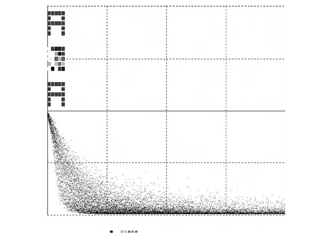
As training proceeds, the program also computes and displays the squared

pattern-matching error

g = enormsq as a function of the trial number t

(Fig. 6-3), with

DOT enormsq = error * error | dispt enormsq

To test the classifier, our experiment protocol restores the data/read pointer

and uses

data/read assignments to feed one pattern at a time directly to the

neural-network input vector

input. No pattern matrix is needed. A second

DYNAMIC program segment labeled

RECALL then runs the neural network

once (

NN = 2) to compute and list the 26 a posteriori probability estimates

p[i] for the first alphabet-letter pattern (Fig. 6-3). Test runs are repeated for

the other letter patterns.

Neural-network Training: Pattern Classification and Associative Memory 137

–

1 1e+04 → 2e+04

scale = 1 ENORMSQ vs. t

FIGURE 6-3. Referring to the softmax pattern-classifier program in Figure 6-2, the bottom

of the display shows superimposed time histories of the squared binary-selector-matching

error

enormsq for all 26 noisy alphabet-letter patterns. The top of the display shows the actual

prototype pattern

input, the noise-corrupted pattern x, and the clean associative-memory out-

put

y for the letter “A”.

6-11. Associative Memory

The

RECALL program segment in Figure 6-2b also computes and displays

the

nx-dimensional pattern yy defined by

Vector yy = INPUT% * p (6-22)

Since

p approximates a binary-selector pattern, yy approximates the prototype

pattern associated with the noise-perturbed input

x (associative memory). Our

RECALL segment also implements a normalized maximum-selecting layer

(Section 6-3)

Vector q^ = v | Vector q = swtch(q) (6-23)

q is necessarily an exact binary-selector pattern, so that the associative-mem-

ory output

Vector y = INPUT% * q (6-24)

reproduces a prototype pattern exactly. Strong noise would cause the selec-

tion of a wrong prototype, but the system is an effective nonlinear noise fil-

ter. Figure 6-3 shows actual patterns

input, x, yy, and y obtained with

moderate noise in the training and recall runs.

NONLINEAR MULTILAYER NETWORKS

6-12. Backpropagation Networks

(a) The Backpropagation Algorithm

We now turn to nonlinear multilayer networks, say a two-layer network

defined by

Vector v1 = tanh(W1 * x)

Vector y = tanh(W2 * v1) (6-25)

The

v1 layer is a hidden layer. For mean-square regression (Section 6-6),

we are given a training sample of paired of nx-dimensional patterns x and

138 Vector Models of Neural Networks

Three layers if the input buffer is counted as an extra layer, as many textbooks do.

Backpropagation networks can also serve as pattern classifiers with a softmax output layer in

the manner of Section 6-10 (Example

ex6-1.lst in the book CD).

ny-dimensional “target” patterns Y. We want to generate ny-dimensional out-

put patterns

y = y(x) that minimize the sample average of

g = ||y(x) –Y||

≡



k=1

(y[k] – Y[k])

(6-26)

Pattern classification can be programmed as mean-square regression on

binary selector patterns, with a softmax output layer as in Section 6-10

(example

bpsoft7.lst in the book CD).

To minimize the mean-square regression error, we update the connection

weights

W1[i, k] and W2[i, k] with a generalized version of the LMS algo-

rithm (6-18), the generalized delta rule

W1[i, k] = W1[i, k] –

ᎏ

lrate1

∂

W1[i, k]

(i = 1, 2, ..., nv1; k = 1, 2, ..., nx)

W2[i, k] = W2[i, k] –

ᎏᎏ

ᎏ

lrate2

∂

W2[i, k]

(i = 1, 2, ..., ny; k = 1, 2, ..., nv1) (6-27)

This is a system of difference equations similar to those in Section 3-1; the

connection weights are difference-equation state variables. The right-hand

side of each difference equation (6-27) is a function of the current values of

the connection weights and defined variables (6-25).

We first compute these defined variables. The derivatives in Eq. (6-27) are

then evaluated by the chain rule. This rather lengthy derivation [7,8] is sim-

plified if we specify intermediate results in terms of three new defined-vari-

able vectors

error, delta1, and delta2 declared with

ARRAY error[ny], delta1[nv1], delta2[ny]

In the DYNAMIC program segment, we program

Vector error = Y – y

Vector delta2 = error * (1 – y^2)

Vector delta1 = W2% * delta2 * (1 – v1^2) (6-28)

in that order (note that

error is defined as in Section 6-10), and then update

the connection-weight matrices with

DELTA W1 = lrate1 * delta1 * x

DELTA W2 = lrate2 * delta2 * v1

(6-29)

Nonlinear Multilayer Networks 139

lrate1 and lrate2 are positive, suitably decreasing learning rates similar to

lrate in Section 6-9. Reference [7] suggests lrate1 = r * lrate2 with r between

2 and 5. Generalization to three or more layers is not difficult.

Most

backpropagation networks have only two layers, and the output layer is often

simply a linear layer.

Neuron layers can be given bias inputs in the manner

of Section 6-2.

Note that

A% denotes the transpose of a matrix A (Section 3-3), products

of two vectors represent matrices (Section 3-10), and the function

1 – Q

the derivative of the neuron activation function

Q = tanh(q).

Interestingly, one can consider the defined-variable assignments (6-28) as

the definition of a neural network that “backpropagates” output-error effects

to the connection weights in each layer of the original neural network.

(b) Discussion

With enough neurons in the first layer, even a two-layer network is theoreti-

cally a “universal approximator,” that is, an output activation

y[i] can

approximate any desired continuous function of the inputs

x[k] [7,8].

Typically, there is more than one optimal set of connection weights. If too

many hidden-layer neurons are used, one might match the training-sample

pairs accurately but make matches for new test samples worse (“overtrain-

ing” hurts “generalization”). This problem is treated in substantial detail in

References [11] and [32].

Unfortunately, backpropagation training is often slowed by flat spots and/or

stopped by local minima in the mean-square error function. A frequently use-

ful partial fix (momentum learning) declares two extra state-variable matrices

140 Vector Models of Neural Networks

The way to add more layers can be seen from the program for a three-layer network with two

hidden layers:

Vector v1 = tanh(W1 * x)

Vector v2 = tanh(W2 * v1)

Vector y = tanh(W3 * v2)

Vector error = Y – y

Vector delta3 = error * (1 – y^2)

Vector delta2 = W3% * delta3 * (1 – v2^2)

Vector delta1 = W2% * delta2 * (1 – v1^2)

DELTA W1 = lrate1 * delta1 * x

DELTA W2 = lrate2 * delta2 * v1

DELTA W3 = lrate3 * delta3 * v2

Example bptest2.lst in the book CD shows the time histories of some hidden neurons in a

three-layer backpropagation network.

In this case, the activation-function derivative factor (1 – y^2) in Eq. (6-28) is omitted, since

all its vector components equal 1.

Dw1, Dw2 and replaces the two matrix difference equations (6-29) with four

difference equations

MATRIX Dw1 = lrate1 * delta1 * x + mom1 * Dw1

MATRIX Dw2 = lrate2 * delta2 * v1 + mom2 * Dw2

DELTA W1 = Dw1 | W2 = Dw2 (6-30)

which make the connection-weight adjustments favor the directions of past

successes. The optimization parameters

mom1, mom2 must be found by trial

and error and are typically between 0.1 and 0.9. There are literally hundreds

of papers and several books [6–9,12–18] describing other improved back-

propagation algorithms, but none work every time. References [2–5] describe

more advanced numerical function-optimization schemes applicable to mul-

tilayer networks. In practice, the best algorithm for a specific application

must be selected (and possibly redesigned) by trial and error. The

Levenberg–Marquart algorithm [5,7] is often a good compromise.

Backpropagation regression networks with a few inputs and one or more out-

puts are used to model empirical relations. As a simple example, the program

in Figure 6-4a trains a two-layer regression network to produce a very accu-

rate sine function; Figure 6-4b shows results. We have defined the two-layer

neural network as a reusable submodel (Section 3-17) in the experiment-

protocol script. The same submodel is then invoked in two separate

DYNAMIC program segments, one for training and one for recall tests. Our

submodel could also be stored and used in another program, say, in a control-

system simulation.

Figure 6-4c shows the squared-error time histories for 32 output activa-

tions of a two-layer, 32-input backpropagation network with

nv = 9 hidden-

layer neurons during a successful training run of

NN = 200,000 steps. A

2.4-GHz personal computer trained 585 connection and bias weights to pro-

duce this display in 7.3 s. The same run took 5.5 s with the display turned off.

6-13. Radial-basis-function Networks

(a) Basis-function Expansion and Linear Optimization

Given a sample of corresponding measurements x, Y, traditional statistical

regression methods have long approximated mean-square regression func-

tions

y(x) (Section 6-6) with weighted sums y(x) = W1 f1(x) + W2 f2(x) + …+

Wn fn(x)

of conveniently chosen basis functions f1(x), f2(x), …, fn(x).One

Nonlinear Multilayer Networks 141