Langetepe E., Zachmann G. Geometric Data Structures for Computer Graphics

Подождите немного. Документ загружается.

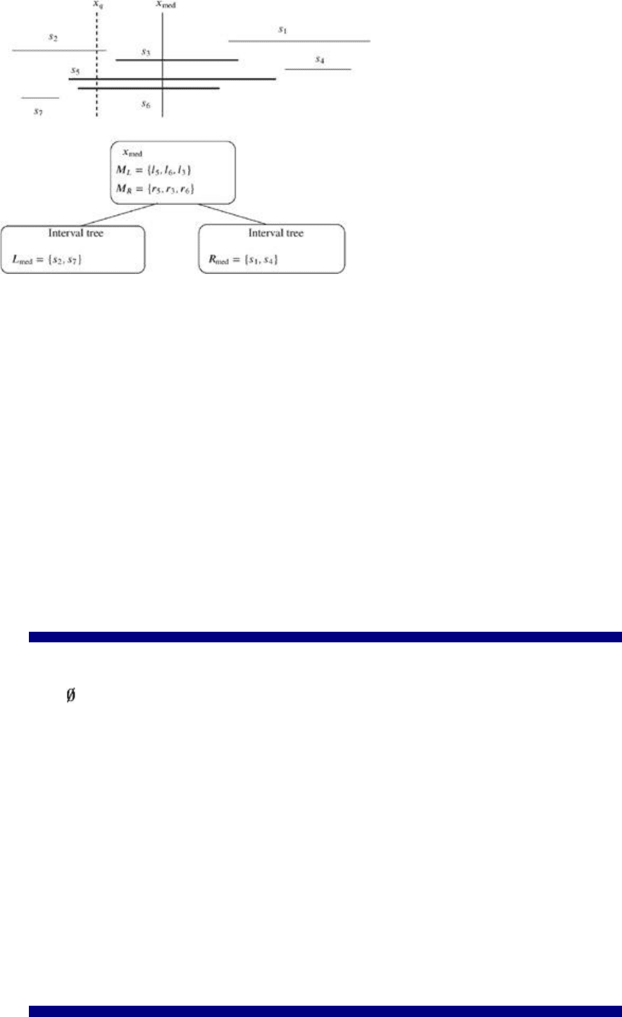
Figure 2.1: An example of the node information in an interval tree. For convenience, the intervals are

represented by 2D line segments. The left and right endpoints l

and r

of the segments s

hit by the

median x

med

are represented in sorted lists M

and M

, respectively.

We construct a data structure that answers the above query efficiently. The information of the intervals

are stored in a binary tree. Let S denote a set of n intervals [l

, r

] for i = 1,

…

, n. The binary interval tree is

constructed recursively, as shown in the construction sketch. A node of the tree is dedicated to a median

value of the endpoint of all segments. For all segments that contain this value, there are two lists for

checking wether a query value is also covered by those intervals; see Figure 2.1 for an example of the

node information. The query operation will be explained in detail later in this chapter.

The following is the interval tree construction algorithm sketch (see also Algorithm 2.1):

 Input: given a set of intervals S represented by [l

, r

] for i = 1,

…

, n;

 If S is empty, then the interval tree is an empty leaf. Otherwise, allocate a node v with two children;

 For the node v, compute the median x

med

of {l

…

, l

, r

…

, r

}. This means that half of the interval

endpoints lie to the left and half of the interval endpoints lie to the right of x

med

. Note that the median

normally will not be equal to a value l

or r

;

 Let L

med

denote the set of intervals to the left of x

med

, let S

med

denote the set of intervals that contain

med

, and let R

med

denote the set of intervals to the right of x

med

;

Algorithm 2.1: Computing an interval tree for a set of intervals, recursively.

IntervalTree(S) (S is a set of intervals {[l

…

, [l

]} together with sorted lists for {l

}, {r

}, and {l

} ∪

})

if S = then

return Nil

else

v := new node

v.S

med

:= HitSegments(v.x

med

,S)

v.x

med

:= Median(S)

med

:= RightSegments(v.x

med

,S)

med

:= LeftSegments(v.x

med

,S)

v.M

:= SortLeftEndPoints(v.S

med

)

v.M

:= SortRightEndPoints(v.S

med

)

v.LeftChild := IntervalTree(L

med

)

v.RightChild := IntervalTree(R

med

)

return v

end if

 At the root v, store x

med

and build a sorted list M

for all left endpoints of S

med

and a sorted list M

for

all right endpoints of S

med

;

 Build the interval trees for L

med

and R

med

recursively for the children of v.

Algorithm 2.1 computes the interval tree efficiently, as shown in Lemma 2.1.

Lemma 2.1. The interval tree for a set S of n intervals has size O(n) and can be constructed in O(n log n)

time.

Proof: In a preliminary step, we sort the interval endpoints by l

order, by r

order, and by total (l

and r

)

order. Obviously, the depth of the constructed tree is in O(log n). Let n

denote the number of intervals at

node v. Computing the median takes O(n

) time using the total order of the interval endpoints. Let m

= |

med

| for the set of intervals S

med

at v. Computing M

and M

from the l

and r

order takes at most O(m

)

time. Since all occurring sets S

med

are distinct, this gives O(n) altogether. Maintaining the l

, r

, and total

order for the recursive steps takes O(n

) time. Altogether, with the recursive steps, we have the recursive

cost function . Together with the depth O(log n) of the tree, we conclude

the given result.

Next, we consider the recursive stabbing query operation for a value x

∈ and the root v of the interval

tree. The median x

med

of node v is used for binary branching. The node information is used for answering

the stabbing query for the intervals that contain the median.

Algorithm 2.2: Answering a stabbing query for an interval tree v and a value x

, recursively.

IntervalStabbing(v, x

) (v is the root of an interval tree, x

∈ )

D := new list

if v.x

med

< x

then

L := v.M

f := L.First

while f ≠ Nil and f < x

D.ListInsert(Seg(f))

f := L.Next

end while

:= IntervalStabbing(v.LeftChild, x

)

else if v.x

med

≥ x

then

R := M

(v)

l := R.Last

while l ≠ Nil and l > x

D.ListInsert(Seg(l))

l := R.Prev

end while

:= IntervalStabbing(v.RightChild, x

)

end if

D := D. ListAdd(D

)

return D

The following is the stabbing query operation sketch:

 Input: given the root v of an interval tree and the query point x

∈ ;

 If x

< x

med

then

o Scan the sorted list M

of the left endpoints in increasing order and report all stabbed segments.

Stop if x

is smaller than the current left endpoint;

o Recursively, continue with the interval tree of L

med

;

 If x

> x

med

then

o Scan the sorted list M

of the right endpoints in decreasing order and report all stabbed

segments. Stop if x

is bigger than the current right endpoint;

o Recursively, continue with the interval tree of R

med

For example, assume that there is a stabbing query at a node v as pointed out in Figure 2.1. Starting from

the left with M

, the segments s

and s

are reported since x

lies to the right of l

and l

. Then the

stabbing query recursively goes on with L

med

and will find s

Lemma 2.2. An (interval/point) stabbing query with an interval tree for a set S of n intervals and a value x

∈ report all k intervals I of S with x

∈ I in O(k + log n) time.

Proof: Scanning through M

or M

at node v takes time proportional to the number of reported stabbed

intervals because we stop as soon as we find an interval that does not contain the point x

. The sets S

med

of all v are distinct, which gives O(k) for all scannings. The size of the considered subtree is divided by at

least two at every level, which gives O(log n) for the path length. Altogether, the given bound holds.

The interval tree was considered in [Edelsbrunner 80] and [McCreight 80]. Note that the interval tree has

no direct generalization to higher dimensions, but can support combined queries; see Section 2.6.

A WeakDelete operation for a segment s (see Chapter 10) can be done in O(log n) time. We find the

corresponding node with s ∈ S

med

and mark the endpoints as deleted in the sorted lists M

and M

Lemma 2.3. A WeakDelete operation for a segment s in an interval tree of n intervals is performed in

O(log n) time.

2.2. Segment Trees

A segment tree is constructed for answering the following 2D (line segment/line) stabbing query

efficiently:

 Input: a set S of segments in the plane;

 Query: a vertical

[1]

line l;

 Output: all segments s ∈ S crossed by l.

Let S = {s

, s

…

, s

} be the set of segments and let E be the sorted set of x-coordinates of the

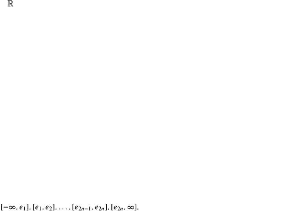
endpoints. We assume general position; that is, E = {e

, e

…

, e

} with e

< e

for i < j (Section 9.5). For

the construction of the tree, we can split E into 2n + 1 atomic intervals

which represent the leaves of the segment tree.

The segment tree is a balanced binary tree. Each internal node v represents an elementary interval I,

which is split into intervals I

and I

for the two children of v. The intervals are split with respect to the

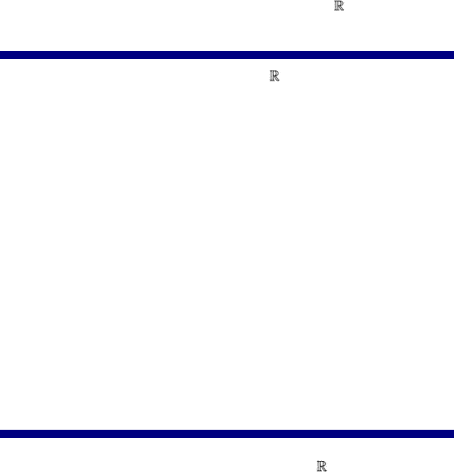
endpoints of the segments; see Figure 2.2. In the first place, the segment tree is a one-dimensional

search tree for the x-coordinates of the endpoints of the segments. The one-dimensional search tree

contains search keys in every node; the data points are represented in the leaves of the tree. Every node

v additionally represents an interval I

so that all points in the (sub)tree represented by root node v are in

. In Section 2.5, we generalize the one-dimensional search tree to arbitrary dimension d. An example of

a one-dimensional search tree is given in Figure 2.7.

Figure 2.2: A segment tree for a set of segments. The segment s is minimally covered by the nodes v

, v

, and v

The following is the one-dimensional search tree sketch (see also Algorithm 2.3):

 Input: given a sorted list S of n elements x

, x

…

, x

;

 Output: the root node of a one-dimensional search tree for S;

 If |S| = 0, then set v := Nil and return v;

 Otherwise, if |S| ≥ 1 then

Algorithm 2.3: Construction of a simple balanced one-dimensional search tree.

SearchTree(S) (S is a sorted list {x

…

, x

})

if S = then

v := Nil

else

v := new node

n := |S|

(L, R) := S. Split(m)

v. Key := S. Get(m)

v.I := [S. First, S. Last])

/* Alternatively: v.I := [x

…

, x

]*/

v. LeftChild := SearchTree(L)

v. RightChild := SearchTree(R)

end if

return v

 Allocate a node v with two children for the root of the tree;

 Choose the element x

of S with and insert the branch key x

at v. Insert the interval I =

, x

] at v. If necessary, I also contains the data points of the interval;

 Compute a one-dimensional search tree v

for x

…

, x

and compute a one-dimensional search tree

for x

m+1

…

, x

;

 Insert v

as the right child of v and v

as the left child of v;

 Finally, return the node v.

Obviously, the corresponding one-dimensional tree has height O(log n). We can find an element x

logarithmic time by starting from the root and branching towards x

using the keys in the nodes. The

sketch and the pseudocode of this simple query procedure are omitted.

So far, we have constructed a tree that represents the information of the end-points of the segments plus

the dummy nodes ∞ and −∞. Obviously, this is not sufficient for answering a stabbing query.

Additionally, we have to incorporate the information of the segments into the tree. Therefore, let us

consider a single segment s represented by the x-coordinates (e

, e

) of its endpoints. The segment s can

be represented by a consecutive set of elementary intervals. We choose a minimal set of elementary

intervals (or the corresponding nodes) in the one-dimensional search tree so that s is fully covered. Due

to Algorithm 2.3, every node represents an elementary interval v.I and, if necessary, its data points.

Minimal means that the nodes are chosen as close as possible to the root of the tree; see Figure 2.2. We

store s in each of the associated nodes. More precisely, let v .pred be the predecessor of v in the interval

tree. A segment s = (e

, e

) represented by the x-coordinates of the endpoints is stored in a list v. L at v iff

v.I ⊆ [e

, e

] and (v.pred). I [e

, e

]. Thus, each node represents an elementary interval v.I and a list of

segments v.L; for an example, see Figure 2.3.

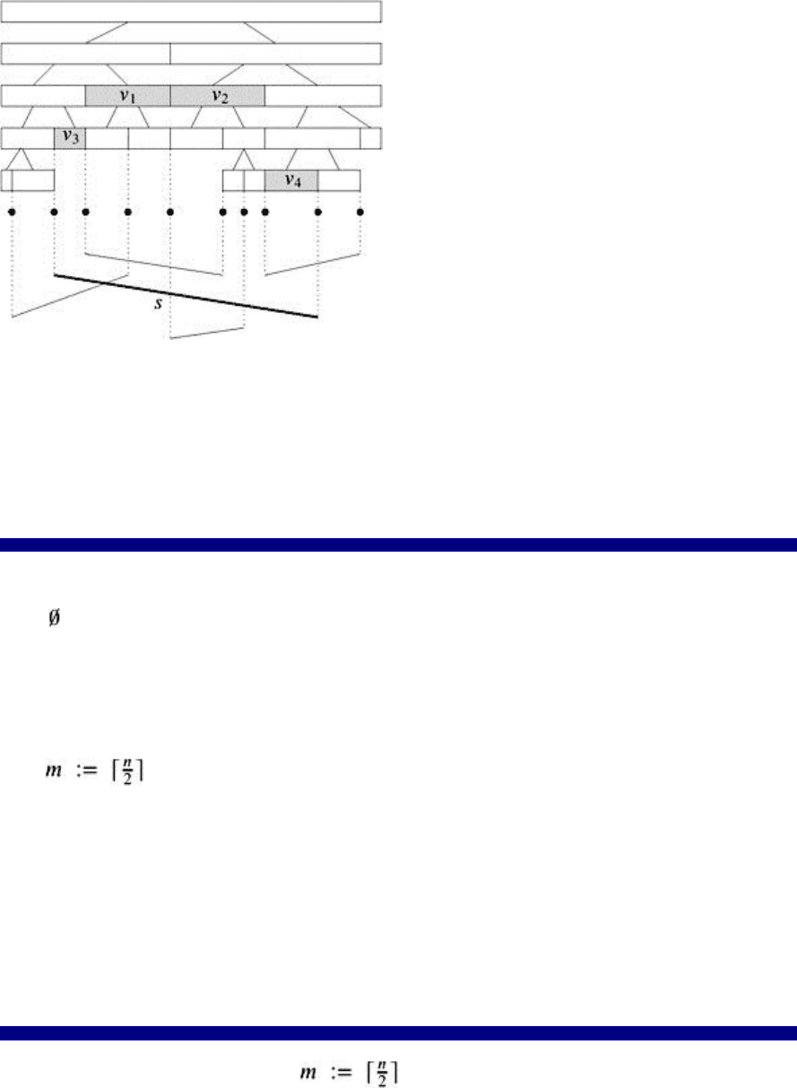
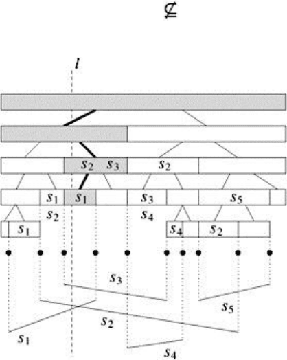
Figure 2.3: The query procedure for a segment tree and a query line l. The shaded intervals indicate the

query path from the root to the leaf. All segments stored at the corresponding nodes are reported.

The one-dimensional search tree with intervals v.I is built up in O(n log n) time, as was shown previously.

However, we need to show how the segment partitions are inserted into the tree. This is done by the

following recursive insert procedure, which has to run for every segment s = (e

, e

The following is the sketch of the segment insertion in the one-dimensional search tree:

 Input: given a line segment s = (e

, e

) and the root v of the segment tree;

 If the interval v.I is already a subset of the interval [e

, e

], then insert s into the segment set v.L and

stop;

 Otherwise, let v. LeftChild and v. RightChild be the children of v. This means that the interval v.I

equals (v.LeftChild).I ∪ (v. RightChild).I;

o If the interval [e

, e

] and the set (v. LeftChild).I overlap, then run the insert procedure

recursively with s and the segment tree v. LeftChild;

o If the interval [e

, e

] and the set (v. RightChild).I overlap, then run the insert procedure

recursively with s and the segment tree v. RightChild.

By inserting every segment into the one-dimensional search tree of the line segment‘s endpoints, we will

finally obtain the segment tree. Altogether, Algorithm 2.4 constructs the segment tree by using Algorithm

2.5 as a subroutine. Note that S

. Extend extends S

by the dummy elements ∞ and −∞.

Lemma 2.4. The segment tree for n segments can be built in O(n log n) and uses O(n log n) space.

Proof: The binary tree has depth O(logn) and O(n) nodes. At each level of the segment tree T, a segment

s = (e

, e

) is stored at most twice. To prove this fact, let us assume that three nodes u

, u

, and u

of the

same level in T contain the segment s. The intervals of their parents do not overlap. This is because they

can overlap only if a pair of u

, u

, and u

has a common predecessor. In this case, the segment has to be

inserted for the predecessor. If the intervals of the parents of u

, u

, and u

do not overlap, the

intermediate node of u

, u

, and u

must have a parent whose interval fully contains [e

, e

]; therefore, s is

not inserted at u

which gives a contradiction. Summing up over all segments and levels, the segment

tree has space O(n log n).

Algorithm 2.4: Building a segment tree.

SegmentTree(S) (S is a set of line segments given by endpoints)

:= S. SortX

:= S

. Extend

v := SearchTree(S

)

while s ≠ do

s := S. First

SegmentInsertion(v, s)

S. DeleteFirst

end while

With a similar argument, one can prove that, during the insertion operation, only four nodes on every level

could be visited. Thus a single segment is inserted in O(log n) time, which gives the overall time bound.

For a stabbing query with a vertical line l, we will proceed as follows. We start with the x-coordinate l

the vertical line l and the root node v of a segment tree.

Algorithm 2.5: Insertion of a segment s in the segment tree.

SegmentInsertion(v, s) (v is one-dimensional search tree of the x-coordinates of the endpoints of segment

set S, s ∈ S.)

:= s. LeftXCoord

:= s. RightXCoord

if v.I ⊂ [e

, e

] then

(v.L). ListAdd(s)

else

if (v. LeftChild).I ∩ [e

, e

] ≠ then

SegmentInsertion(v. LeftChild, s)

end if

if (v. RightChild).I ∩ [e

, e

] ≠ then

SegmentInsertion(v. RightChild, s)

end if

Algorithm 2.6: The stabbing query for a segment tree.

StabbingQuery(v, q) (v is the root node of a segment tree and l a vertical line segment)

L := Nil

if v ≠ Nil and l

∈ v.I then

L := v.L

:= StabbingQuery(v. LeftChild, l)

:= StabbingQuery(v. RightChild, l)

L. ListAdd(L

)

L. ListAdd(L

)

end if

return L

The following is the sketch of the stabbing query with a segment tree:

 Input: given the x-coordinate l

of the vertical line l and the root node v of a segment tree;

 If l

is inside the interval v.I, then report all segments in v.L;

 If v is not a leaf, then for the children v. LeftChild and v. RightChild of v, we know that the interval v.I

equals (v. LeftChild).I ∪ (v. RightChild).I and we proceed as follows:

o If l

lies inside (v. LeftChild).I, then start a query with segment tree v. LeftChild and l

;

o Else we have l

∈ (v. RightChild).I, and we start a query with segment tree v. RightChild and l

Figure 2.3 shows an example for a segment query. The shaded intervals indicate the query path from the

root to the leaf.

Lemma 2.5. A vertical line stabbing query for n segments in the plane can be answered by a segment

tree in time O(k + log n), where k stands for the number of reported segments.

Proof: Obviously, the tree is traversed with O(log n) steps. The running time O(k + log n) stems from the

cardinality k of the corresponding sets v.L.

The segment tree was first considered in [Bentley 77] and extended to higher dimensions by several

authors; see, for example, [Edelsbrunner and Maurer 81] and [Vaishnavi and Wood 82].

A WeakDelete operation can be performed in O(log n) time (see Chapter 10). We have to mark a

segment s in every list v.L with s ∈ v.L. By construction, a segment s is stored at most twice in every level

of the segment tree and occurs at most O(log n) times. We proceed as if we would like to insert the

segment s, which can be done in O(log n) time; see also the proof of Lemma 2.4.

Lemma 2.6. A WeakDelete operation for a segment tree of n segments in the plane can be performed in

time O(log n).

[1]

Arbitrary query lines l can be handled by application of a transformation matrix; see Section 9.5.3.

2.3. Multi-Level Segment Trees

In the preceding sections, we considered segment trees for 2D objects. Now, we generalize the

approach. Namely, we consider the following multi-dimensional stabbing problem and make use of a set

of inductively defined segment trees. Multi-level segment trees support (axis-parallel box/point) stabbing

queries as follows:

 Input: a set S of n axis-parallel boxes in ;

 Query: a query point q in ;

 Output: all boxes B ∈ S with q ∈ B.

This stabbing query has many applications in computer graphics. For example, objects in the sphere may

be approximated by their axis-parallel bounding box. For every point q, the (bounding box/point) stabbing

query will report all objects that are near q. Figure 2.4 shows a simple example in 2D.

Figure 2.4: A stabbing query for a set of bounding boxes can report all polygonal objects near q.

A single d-dimensional box B

can be defined by a set of d axis-parallel segments

starting at a unique corner ; see Figure 2.5 for a 2D example. A multi-level

segment tree T

with respect to (x

, x

…

, x

), where x

denotes the ith coordinate, is inductively defined.

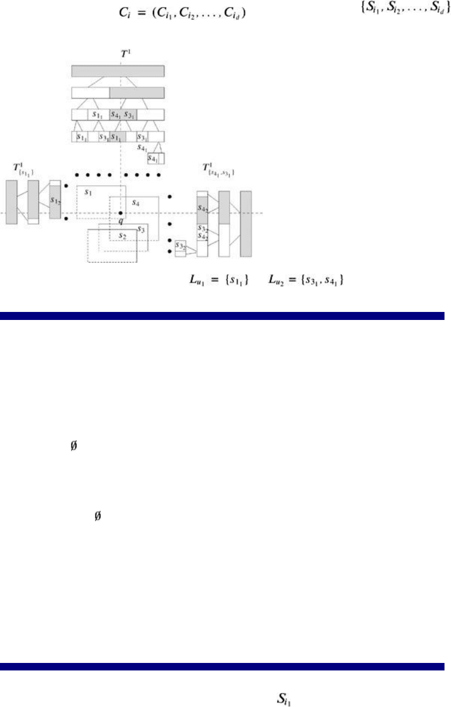
Figure 2.5: Some parts of the multi-level segment tree of four boxes in 2D. The segment tree T

and the

relevant trees for the nodes u

and u

with and for the query point q are

shown.

Algorithm 2.7: The inductive construction algorithm of a multi-level segment tree.

MLSegmentTree(B, d) (B is a set of boxes in dimension d; each box is represented by a set of line

segments)

S := B. FirstSegmentsExtract

T := SegmentTree(S)

T. Dim := d

if d > 1 then

N := T.GetAllNodes

while N ≠ do

u := N. First N. DeleteFirst

L := u.L

B := new list

while L = do

s := L. First L. DeleteFirst

B := B. ListAdd( s. Box(d − 1))

end while

u. Pointer := MLSegmentTree(B, d − 1)

B. Deallocate

end while

end if

return T

The following is the multi-level segment tree construction sketch:

 Build a one-dimensional segment tree T

for all segments with respect to the x

coordinate;

 For every node u of T

o Build a (d − 1)-dimensional multi-level segment tree for the set of boxes

where u.L denotes the set of segments stored at u in T

;

o Associate a pointer in T

from u to .

A query is answered recursively in a straightforward manner. If a set of segments in dimension j has to be

reported, we recursively check the corresponding tree with dimension j − 1. The corresponding box is

reported only if the query succeeds in every dimension. This means that finally we get an answer for a

tree .

Algorithm 2.8: The inductive query operation for a multi-level segment tree.

MLSegmentTreeQuery(T, q, d) (q ∈ , T is the root node of a d-dimensional multi-level segment tree)

if d = 1 then

L := StabbingQuery(T, q)

A := L. GetBoxes

else

A := new list

L := SearchTreeQuery(T, q.First)

while L ≠ do

t := (L. First). Pointer

B := MLSegmentTreeQuery(t, q. Rest, d − 1)

A. ListAdd(B)

L. DeleteFirst

end while

return A

end if

More precisely, a query for a query point q = (q

, q

…

, q

) and a multi-level segment tree T

for a set of

segments S

…

, S

is given in the following sketch.

The following is the multi-level segment tree query sketch:

 If d = 1, answer the question with the corresponding segment tree T

; see Algorithm 2.6 and return

the boxes associated to the segments reported;

 Otherwise, traverse T

and find the nodes u

…

, u

so that q

lies in the intervals (u

).I of the nodes u

of T

for i = 1 to l;

 For 1 ≤ i ≤ l, answer recursively the query (q

…

, q

) for the tree of the set of segments (u

).L stored at u

, respectively.

The following time and space bounds hold.

Theorem 2.7. A multi-level segment tree for a set of n axis-parallel boxes in dimension d can be built up

in O(n log

n) time and needs O(n log

n) space. A (axis-parallel box/point) stabbing query can be

answered in O(k + log

n) time.

Proof: First, we sort the segment endpoints with respect to every dimension. The first segment tree T

built up in O(n log n) time, occupies space O(n log n), and has O(n) nodes. Next, we construct (d − 1)-

dimensional segment trees for the set v.L of every node v in T

. By induction, we can assume that the (d

− 1)-dimensional segment tree for a node v ∈ T

with |v.L| segments is computed in O(|v.L| log

(d−1)

|v.L|).

Additionally, as already proven, every segment s

occurs in O(log n) lists v.L, i.e., in O(log n) (d − 1)-

dimensional segment trees. This means that is in O(n log n), and the overall running time is

given by

The required space can be measured as follows. The whole structure T

consists of one-dimensional

segment trees T

only. In how many trees will a part of the box B

appear? In the first tree T

, the segment

of the box B

appears in O(log n) nodes. Therefore, it appears in O(log n) trees . In each of

these trees, the segment of the box B

appears again in O(log n) nodes. Altogether, segments of B

appear in

nodes. Summing up over all n segments gives O(n log

n) entries. By the same argument, the number of

trees is bounded by O(log

n) also, so that the number of empty nodes is in O(n log

n).

Analogously, a query traverses along O(log

n) nodes. For the first tree T

, the query traverses O(log n)

nodes and therefore O(log n) new queries have to be considered. Recursively, O(log n) nodes in O(log n)

new trees may be traversed. In the final segment trees, k boxes may also be reported. Altogether

nodes are visited, and the running time for a query is O(k + log

n).

A WeakDelete operation (see Chapter 10) for a segment s in the multi-level segment tree can be

performed in O(log

n) time due to the number of nodes where s appears and due to the time for visiting

all these nodes. Technically, we can reinsert the segment s recursively into the multi-level segment tree.

Lemma 2.8. A WeakDelete operation for a d-dimensional multi-level segment tree for a set of n axis-

parallel boxes can be performed in time O(log

n).

Next, we turn to the subject of orthogonal windowing queries.

2.4. Kd-Trees

In general, a windowing query considers a set of objects and a multi-dimensional window, such as a box.

All objects that intersect with the window should be reported. Thus, one can easily decide which objects

are located within a certain area, one of the classic problems arising in computer graphics.

The kd-tree is a natural generalization of the one-dimensional search tree considered in the previous

section. It can be viewed also as a generalization of quadtrees. With the help of a kd-tree, one can

efficiently answer (point/axis-parallel box) windowing queries as follows:

 Input: a set of points S in ;

 Query: an axis-parallel d-dimensional box B;

 Output: all points p ∈ S with p ∈ B.

Let D be a set of n points in . For convenience, we assume that for a while k = 2, and that all x- and y-

coordinates are different. If this is not the case, we will have a so-called degenerate situation, and we can

apply the techniques presented in Section 9.5. Let us further assume that we have decided to split D

along the x-axis, and that we have determined the split value s of the x-coordinates. Then we split D by

the split line x = s into subsets