Lazinica A. (ed.) Particle Swarm Optimization

Подождите немного. Документ загружается.

Using Opposition-based Learning with Particle Swarm Optimization

and Barebones Differential Evolution

381

opposition-based learning improved the performance of both PSO and BBDE without

requiring any extra parameter.

PSO iPSO

Sphere 0(0) 0(0)

Rosenbrock

22.191441

(1.741527)

20.645323

(0.426212)

Rotated hyper-

ellipsoid

2.021006

(1.675313)

0.355572

(0.890755)

Rastrigin

48.487584

(14.599249)

27.460845

(11.966896)

Ackley

1.096863

(0.953266)

0(0)

Griewank

0.015806

(0.022757)

0.006163

(0.009966)

Salomon

0.446540

(0.122428)

0.113207

(0.034575)

Table 1. Mean and standard deviation (±SD) of the function optimization results

BBDE iBBDE

Sphere 0(0) 0(0)

Rosenbrock

25.826400

(0.216660)

25.942146

(0.209437)

Rotated hyper-

ellipsoid

15.409460

(20.873456)

0.905987

(1.199178)

Rastrigin

34.761833

(28.598884)

0(0)

Ackley 0(0) 0(0)

Griewank

0.000329

(0.001800)

0(0)

Salomon

0.166540

(0.047946)

0.149917

(0.050826)

Table 2. Mean and standard deviation (±SD) of the function optimization results

Particle Swarm Optimization

382

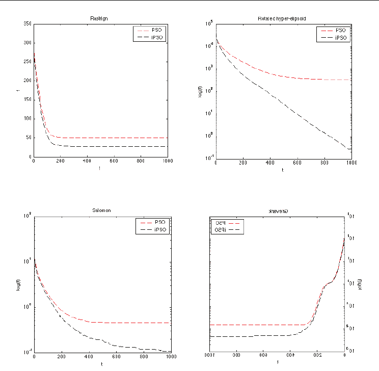
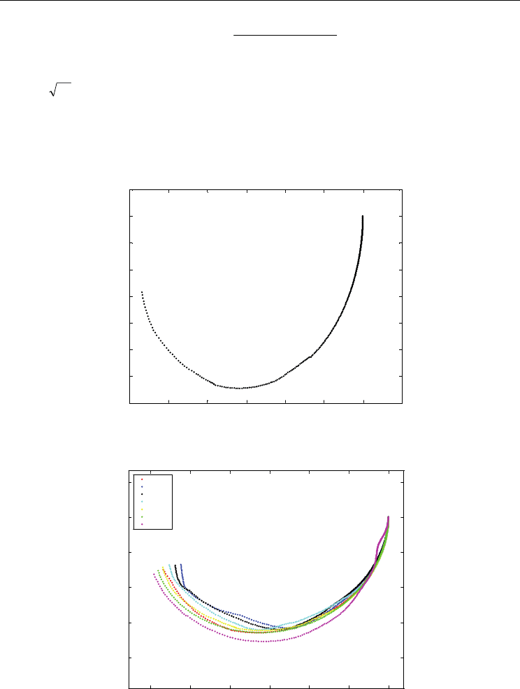
Figure 1. Performance Comparison of PSO and iPSO when applied to selected functions

7. Conclusion

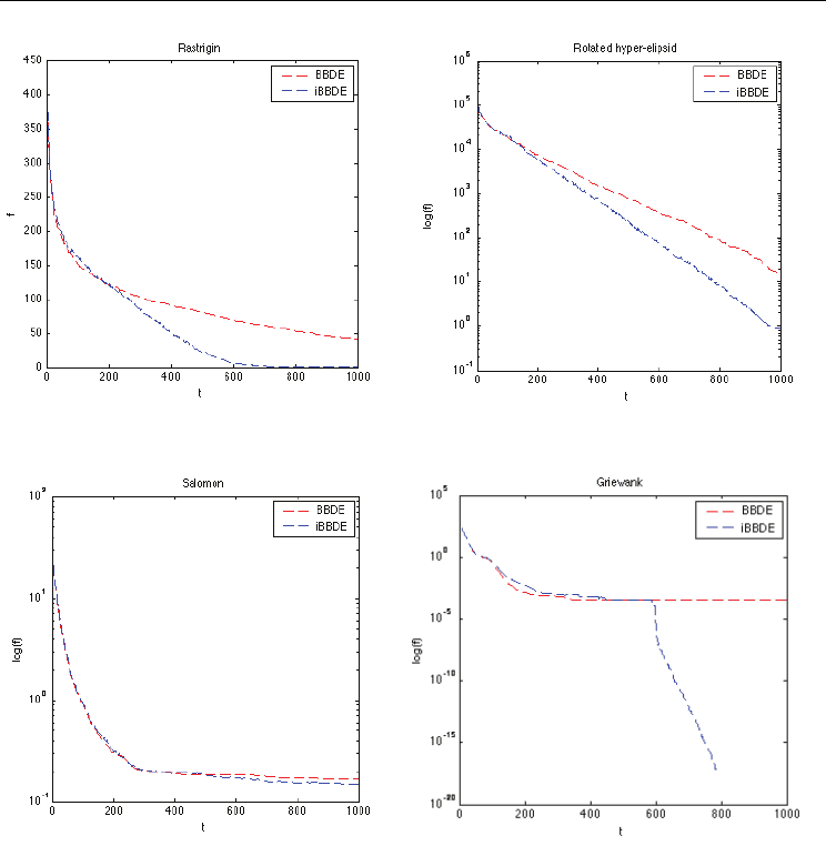
Opposition-based learning was used in this chapter to improve the performance of PSO and

BBDE. Two opposition-based variants were proposed (namely, iPSO and iBBDE). The iPSO

and iBBDE algorithms replace the least-fit particle with its anti-particle. The results show

that, in general, iPSO and iBBDE outperformed PSO and BBDE, respectively. In addition,

the results show that using OBL enhances the performance of PSO and BBDE without

requiring additional parameters. The ideas introduced in this chapter could also be used

with any PSO/BBDE variant.

Future research will investigate the effect of noise on the performance of the proposed

approaches. Furthermore, a scalability study will be conducted. Finally, applying the

proposed approaches to real-world problem will be investigated.

Using Opposition-based Learning with Particle Swarm Optimization

and Barebones Differential Evolution

383

Figure 2. Performance Comparison of BBDE and iBBDE when applied to selected functions

8. References

Clerc, M. & Kennedy, J. (2002). The Particle Swarm-Explosion, Stability, and Convergence in

a Multidimensional Complex Space. IEEE Transactions on Evolutionary Computation,

Vol. 6, No. 1, pp. 58-73.

Engelbrecht, A. (2005). Fundamentals of Computational Swarm Intelligence, Wiley & Sons.

Han, L. & He, X. (2007). A novel Opposition-based Particle Swarm Optimization for Noisy

Problems. Proceedings of the Third International Conference on Natural Computation,

IEEE Press, Vol. 3, pp.

624 – 629.

Particle Swarm Optimization

384

Kennedy, J. (1999). Small Worlds and Mega-Minds: Effects of Neighborhood Topology on

Particle Swarm Performance. Proceedings of the IEEE Congress on Evolutionary

Computation, Vol. 3, pp. 1931-1938.

Kennedy, J. (2003). Bare Bones Particle Swarms. Proceedings of the IEEE Swarm Intelligence

Symposium, pp. 80-87.

Kennedy, J. & Eberhart, R. (1995). Particle Swarm Optimization. Proceedings of the IEEE

International Joint Conference on Neural Networks, pp. 1942-1948.

Kennedy, J. & Mendes, R. (2002). Population Structure and Particle Performance. Proceedings

of the IEEE Congress on Evolutionary Computation, pp. 1671-1676, IEEE Press.

Omran, M., Engelbrecht, A. & Salman, A. (2007). Differential evolution based on particle

swarm optimization. Proceedings of the IEEE Swarm Intelligence Symposium, pp. 112-

119.

Price, K.; Storn, R. & Lampinen, J. (2005). Differential Evolution: A Practical Approach to Global

Optimization, Springer.

Rahnamayan, S.; Tizhoosh, H. & Salama, M. (2008). Opposite-based Differential Evolution.

IEEE Trans. On Evolutionary Computation, Vol. 12, No. 1, pp. 107-125.

Shi, Y. & Eberhart, R. (1998). A Modified Particle Swarm Optimizer. Proceedings of the IEEE

Congress on Evolutionary Computation, pp. 69-73.

Storn, R. & Price, K. (1995). Differential evolution - A Simple and efficient adaptive scheme

for global optimization over continuous spaces. Technical Report TR-95-012,

International Computer Science Institute.

Tizhoosh, H. (2005). Opposition-based Learning: A New Scheme for Machine Intelligence.

Proceedings Int. Conf. Comput. Intell. Modeling Control and Autom, Vol. I, pp. 695-701.

van den Bergh, F. (2002). An Analysis of Particle Swarm Optimizers. PhD thesis, Department

of Computer Science, University of Pretoria, Pretoria, South Africa, 2002.

van den Bergh, F. & Engelbrecht, A. (2006). A Study of Particle Swarm Optimization Particle

Trajectories. Information Sciences, Vol. 176, No. 8, pp. 937-971.

Wang, H.; Liu, Y.; Zeng, S.; Li, H. & Li, C. (2007). Opposition-based Particle Swarm

Algorithm with Cauchy Mutation. Proceedings of the IEEE Congress on Evolutionary

Computation, pp. 4750-4756.

Particle Swarm Optimization: Dynamical

Analysis through Fractional Calculus

E. J. Solteiro Pires

, J. A. Tenreiro Machado

and P. B. de Moura Oliveira

Universidade de Trás-os-Montes e Alto Douro,

Instituto Superior de Engenharia do Porto

Portugal

1. Introduction

This chapter considers the particle swarm optimization algorithm as a system, whose

dynamics is studied from the point of view of fractional calculus. In this study some initial

swarm particles are randomly changed, for the system stimulation, and its response is

compared with a non-perturbed reference response. The perturbation effect in the PSO

evolution is observed in the perspective of the fitness time behaviour of the best particle.

The dynamics is represented through the median of a sample of experiments, while

adopting the Fourier analysis for describing the phenomena. The influence upon the global

dynamics is also analyzed. Two main issues are reported: the PSO dynamics when the

system is subjected to random perturbations, and its modelling with fractional order

transfer functions.

2. Particle Swarm Optimization Basics

Evolutionary algorithms have been successfully applied to solve complex optimization

engineering problems. Together with genetic algorithms, the particle swarm optimization

(PSO) algorithm, proposed by (Kennedy & Eberhart, 1995), has achieved considerable

success in solving optimization problems. While PSO algorithms and related variants have

been extensively studied (Clerk & Kennedy, 2002), the influence of perturbations signals

over the operation conditions is not yet well known.

The PSO algorithm was proposed originally by Kennedy and Eberhart (1995). This

optimization technique is inspired in the way swarms behave and its elements move in a

synchronized way, both as a defensive tactic and for searching food. An analogy is

established between a particle and a swarm element. The particle movement is characterized

by two vectors, representing its current position x and velocity v. Since 1995, many

techniques were proposed to refine and/or complement the original canonical PSO

algorithm, namely regarding it’s tuning parameters (Shi and Eberhat, 1999) and by

considering hybridization with other evolutionary techniques (Lovbjerg et al., 2001).

In this study a standard elementary PSO algorithm is considered (see Fig. 1). The basic

algorithm begins by initializing the swarm randomly in the search space. As it can be seen in

Fig. 1, where t and t + 1 represent two consecutive iterations, the position x of each particle

is changed during the iterations by adding a new velocity v. This velocity is evaluated by

Particle Swarm Optimization

386

summing an increment to the previous velocity value. The increment is a function of two

components representing the cognitive and the social knowledge.

The cognitive knowledge of each particle is included by evaluating the difference between

the current position x and its best position so far b. The social knowledge of each particle is

incorporated through the difference between its current position x and the best swarm

global position achieved so far g. The cognitive and social knowledge factors are multiplied

by randomly uniformly generated terms ϕ

and ϕ

, respectively. The particles velocity is

restricted, in order to keep velocities from exploding, through the inertia term I (Clerk and

Kennedy, 2002).

Initialize Swarm

forAll particles

calculate fitness f

endfor

Repeat

forAll particles

t+1

=Iv

+ϕ

(b-x

)+ ϕ

(g-x

)

t+1

endfor

forAll particles

calculate fitness f

endfor

until Stopping criteria

Figure 1. Particle swarm optimization algorithm

3. Fractional Calculus

Fractional Calculus (FC) goes back to the beginning of the theory of differential calculus.

Nevertheless, the application of FC just emerged in the last two decades, due to the progress

in the area of chaos that revealed subtle relationships with the FC concepts. In the field of

dynamical systems theory some work has been carried out but the proposed models and

algorithms are still in a preliminary stage of establishment.

The fundamentals aspects of FC theory are addressed in (Gement, 1938; Méhauté, 1991;

Oustaloup, 1991; Podlubny, 1999). Concerning FC applications research efforts can be

mentioned in the area of viscoelasticity, chaos, fractals, biology, electronics, signal

processing, diffusion, wave propagation, percolation, modelling, control and irreversibility

(Ross, 1974; Tenreiro Machado, 2001; Torvik, 1984; Vinagre, 2002; Westerlund, 2002).

The FC is a generalization of the classical differential calculus to a non-integer order α ∈ C.

Since its foundation has been the subject of distinct approaches. Due to this reason there are

several alternative definitions of fractional derivatives. For example, the Laplace definition

of a derivative of order α ∈ C of the signal x(t), D

[x(t)], is a ‘direct’ generalization of the

classic integer-order scheme yielding equation (1):

[]

)(})({ sXstxDL

αα

(1)

for zero initial conditions, where s represents the Laplace operator. This means that

frequency-based analysis methods have a straightforward adaptation.

Particle Swarm Optimization: Dynamical Analysis through Fractional Calculus

387

An alternative approach, based on the concept of fractional differential, is the Grünwald-

Letnikov definition given by equation (2) where h represents the time increment.

[]

⎥

⎦

⎤

⎢

⎣

⎡

+−+Γ

−+Γ−

∑

+∞

→

)1)(1(

)()1()1(1

lim)(

khtx

txD

(2)

An important property revealed by equation (2) is that while an integer-order derivative

implies just a finite series, the fractional-order derivative requires an infinite number of

terms. This means that integer derivatives are ‘local’ operators in opposition with fractional

derivatives which have, implicitly, a ‘memory’ of all past events.

The characteristics revealed by fractional-order models make this mathematical tool well

suited to describe phenomena such as irreversibility and chaos, because of its inherent

memory property. In this line of thought, the propagation of perturbations and the

appearance of long-term dynamic phenomena in a population of individuals subjected to an

evolutionary process seems to be a case where FC tools fit adequately, as shown in (Solteiro

Pires et al.; 2003, Solteiro Pires et al., 2006) for genetic algorithms.

4. PSO Swarm Optimization Dynamic analysis

4.1 Problem statement

This section introduces the problem formulation adopted in the study of the PSO dynamic

systems. Moreover, the dynamical phenomena involved in the signal propagation within

the PSO population is analyzed. For a statistical sample of n independent cases, a particle is

randomly initialized, in every experiment, and replaces the corresponding particle of the

initial reference population. The experiments reveal a fractional dynamics of the

perturbation propagation during the evolution which can be described by system theory

tools.

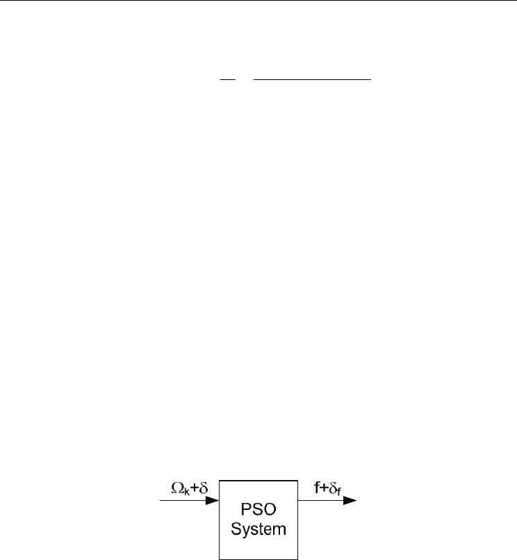
The PSO algorithm, called in this report the ‘system’, is applied in the optimization of: a

quadratic function, the Eason function and the Bohachevsky function.

Figure 2. Perturbation of the PSO system

In the first test function case, the objective function consists in minimizing the quadratic

function (3) which is adopted as a case study due to it’s simplicity.

)f( xx = (3)

This function has only one parameter and its global optimum value is located at f(x)|

opt

= 0.

The variable interval is x ∈ [-100,100] and the algorithm uses an encoding scheme with real

numbers to codify the particles. A PSO is executed during a period of T

= 10000 iterations

with {ϕ

, ϕ

} ~ U[0, 1.5].

Particle Swarm Optimization

388

The influence of several factors can be analyzed in order to study the dynamics of the PSO

system, particularly the inertia factor I or the ϕ

factors, i = {1, 2}. This effect can vary

according to the population size, fitness function and iteration number used. As mentioned

previously, one particle of the initial population is changed randomly. The inertia parameter

influence is studied to analyze the effect of the perturbation for the values of

I = {0.50, 0.55,..., 0.80} versus the swarm population size pop = {6, 8,..., 12}. The variation of

the best global particle fitness evolution is taken as the system output signal as illustrated in

Fig. 2.

4.2 The PSO dynamics

Initially, the PSO system is executed without any initial perturbation signal, during

= 10000 iterations, for a predefined inertia weight value I and swarm population size.

The data regarding this test is stored, namely the global particle fitness and the stochastic

parameters. This experiment will serve as a reference test. The optimization system

perturbation consists in replacing the first initial particle of the stored reference swarm

population, in every algorithm execution, by another particle randomly generated. Indeed,

this stimulus to the system, results in a swarm fitness modification δf which is evaluated.

This perturbation test is repeated for n = 10000 cases. It is important to state that the

remaining test conditions, namely the stochastic reference stored values, remain unchanged

along the n experiments. Therefore, the variation of the resulting PSO swarm fitness

perturbation, during the evolution, can be viewed as the output signal which varies during

the successive iterations.

The output signal consists in the difference between the population fitness with and without

the initial perturbation, that is, δf(T) = f

pert

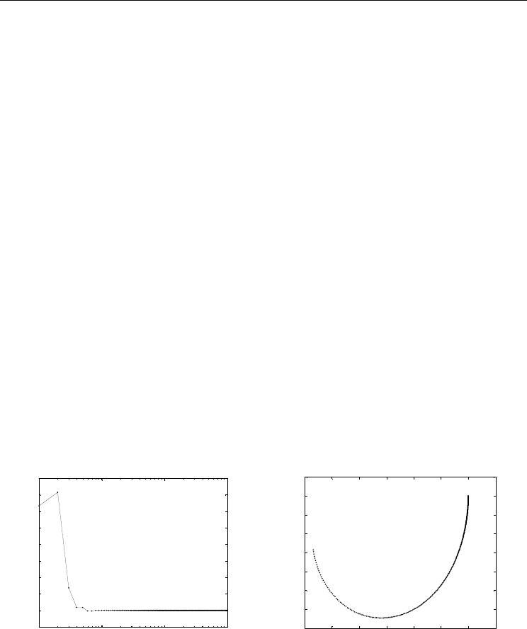
(T) − f(T). Figure 3a) shows the output signal

δ f(T), for one particle replacement, in the iteration domain. In each experiment the Fourier

transform of the signal perturbation, F[δ f(T)] (see Fig. 3b)) is evaluated in order to analyze

the dynamics.

-5

-0.2 0 0.2 0.4 0.6 0.8 1 1.2

-0.7

-0.6

-0.5

-0.4

-0.3

-0.2

-0.1

0.1

ℜ

{H(jw)}

ℑ

{H(jw)}

a) Iteration domain b) Polar diagram

Figure 3. Output signal for an initial perturbation. Experiment with I = 0.7 and a swarm

population size of pop = 12 elements.

With the output signal Fourier description it is possible to evaluate the corresponding

normalized transfer function (4):

Particle Swarm Optimization: Dynamical Analysis through Fractional Calculus

389

)0)}(f({

))}(jf({

)H(j

ωδ

(4)

where w represents the frequency, T the discrete time evolution (number of iterations used)

and

1j −=

. The transfer function H(jw) for this experiment is depicted in Figure 3b).

Finally it is obtained a ‘representative’ transfer function, by using the median of the

statistical sample (Tenreiro Machado & Galhano, 1998) of n experiments (see Figure 4).

Figure 5 shows the archieved results for inertial values of I = {0.50, 0.55,..., 0.80}. The medians

of the transfer functions calculated previously (i.e., for the real and the imaginary parts for each

frequency) are taken as the final result of the numerical transfer function H(jw).

-0.2 0 0.2 0.4 0.6 0.8 1 1.2

-0.7

-0.6

-0.5

-0.4

-0.3

-0.2

-0.1

0.1

ℜ

{H(jw)}

ℑ

{H(jw)}

Figure 4. Median transfer function H(jw) of n = 10000 experiments for an inertial term I = 0.7

and pop = 12 elements.

-0.2 0 0.2 0.4 0.6 0.8 1

-0.8

-0.6

-0.4

-0.2

0.2

ℜ

{H(jw)}

ℑ

{H(jw)}

I=0.50

I=0.55

I=0.60

I=0.65

I=0.70

I=0.75

I=0.80

Figure 5. Median transfer function H(jw), of the n experiments for I = {0.50, 0.55,…, 0.80} for

a population swarm of pop = 12 elements.

Particle Swarm Optimization

390

Varying the swarm population number of elements in the interval pop ∈ [6, 12] results in a

family of transfer functions. For a swarm size greater than 12 elements there is no difference

between the reference test and the perturbation tests. It can be concluded that with large

swarms an element has a negligible impact upon the search and, consequently, the

performance of the algorithm is independent of the initial swarm. On the other hand, in

small swarms, an element has a large impact on the evolution; therefore, it is necessary a

large number of perturbation tests to lead to a convergence towards the statistical sample

median. From the tests it can be observed that for I = 0.8 the median is very irregular

because the system is close to the instability region (den Bergh and Engelbrecht, 2006).

4.3 Dynamical analysis

In this section the median of the numerical transfer functions is approximated by analytical

expressions with gain k = 1 and one pole a ∈ R

of fractional order α ∈ R

, given by equation

(5):

⎟

⎠

⎞

⎜

⎝

⎛

)G(j

(5)

Since the normalized Fourier transform (H) is used, it yields k = 1. In order to estimate the

transfer function parameters {a, α} another PSO algorithm is used, which is named the

identification PSO. The identification PSO is executed during T

ide

= 200 iterations with a 100

particle swarm size. The PSO parameters are: {ϕ

, ϕ

}~U[0, 1.5], I = 0.6, and the transfer

function parameters intervals are a ∈ [4 × 10

-3

, 50] and α ∈ [0, 100].

To guide the PSO search, the fitness function f

ide

is used to measure the distance between the

numerical median H(jw

) and the analytical expression G(jw

∑

−=

ide

)G(j)H(j)(jf

ωωω

(6)

where nf is the total number of sampling points and w

, k = {1,...,nf}, is the corresponding

vector of frequencies.

As explained previously, the optimization PSO has stochastic dynamics. Therefore, every

time the PSO system is executed with a different initial particle replacement, it leads to a

slightly different transfer function. Consequently, in order to obtain numerical convergence

(Tenreiro Machado & Galhano, 1998) n = 10000 perturbation experiments are performed

with different replacement particles, while all the other particles remain unchanged. The

optimization PSO dynamics transfer function is evaluated by computing the normalized

signals Fourier transform (FT) (equation 4). The transfer functions medians determined

previously (i.e., for the real and the imaginary parts, and for each frequency) are taken as the

final result of the numerical transfer function H(jw).

Figure 6 and 7 show, superimposed, the normalized median transfer function H(jw) and the

corresponding identified transfer function G(jw), both as polar and amplitude diagrams,

respectively. As it can be observed from these figures the fractional order transfer function,