Lazinica A. (ed.) Particle Swarm Optimization

Подождите немного. Документ загружается.

Simultaneous Perturbation Particle Swarm Optimization and Its FPGA Implementation

351

particle swarm optimization, left half particles are modified only by the simultaneous

perturbation.

All the individuals select the particle swarm optimization or the simultaneous perturbation

randomly with probability of 0.5 in every iteration.

It is interesting what level of performance does such a simple mixture of the particle swarm

optimization and the simultaneous perturbation has. Changing ratio of the particle swarm

optimization and the simultaneous perturbation is another option.

3.4 Scheme 4

We have another option to construct new algorithm. Basically, we use the algorithm 3.

However, the best individual is updated only by the simultaneous perturbation. The reason

is as same as that of the algorithm 2. The best particle has a good chance to be a neighbor of

a global minimum. Therefore, we always use the simultaneous perturbation for the best

particle.

4. Comparison

In order to evaluate performance of these algorithms, we use the following test functions.

These functions have their inherent characteristics about local minimum or slope.

• Rastrigin function

• Rosenbrock function

• 2

-minima function

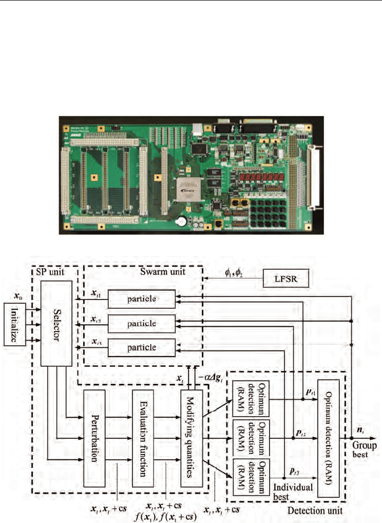
Comparisons are carried out for ten-dimensional case, that is, n=10 for all test functions.

Average of 50 trials is shown. 30 particles are included in the population. Change of average

means that an average of the best particle in 30 particles at the iteration for 50 trials are

shown. For the simultaneous perturbation term, the perturbation c is generated by uniform

distribution in the interval [0.01 0.5] for the scheme 1 to 4. These setting are common for the

following test functions.

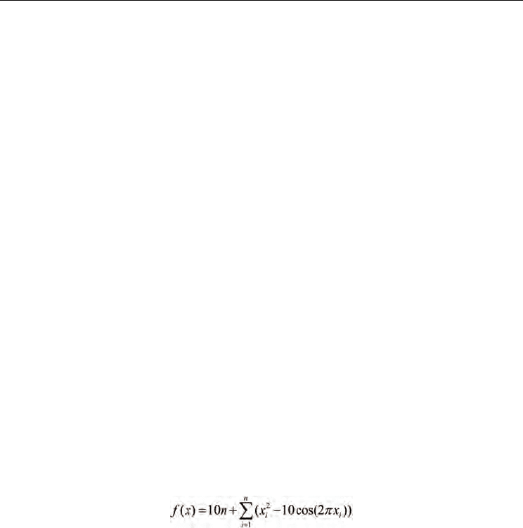
1. Rastrigin function

The function is described as follows;

(6)

The shape of this function is shown in Fig.2 for two-dimensional case. The value of the

global minimum of the function is 0. Searched area is -5 up to +5 for the function. We found

the best setting of the particle swarm optimization for the function

=1.0 and

=0.9.

Upper limitation of

and

are 2.0 and 1.0, respectively. Using the setting (See Table 1),

we compare these four methods and the ordinary particle swarm optimization.

As shown in the figure, this function contains many local minimum points. It is generally

difficult to find a global minimum using the gradient type of the method. It is difficult also

for the particle swarm optimization to cope with the function. The past experiences will not

give any clue to find the global minimum. This is one of difficult functions to obtain the

global minimum.

Change of the best particle is also depicted in Fig.3. The horizontal axis is number of

observations for the function. The ordinary particle swarm optimization requires the same

number of observations with the number of particles in the population. Since the scheme 1

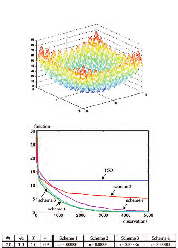
Particle Swarm Optimization

352

contains the simultaneous perturbation procedure, the scheme uses twice number of the

observations. However, this does not change, even if the dimension of the parameters

increases.

Figure 2. Rastrigin function

Figure 3. Change of the best particle for Rastrigin function

Table 1. Parameters setting for Rastrigin function

Simultaneous Perturbation Particle Swarm Optimization and Its FPGA Implementation

353

The scheme 2 has the number of the observations of the ordinary particle swarm

optimization plus one, because only the best particle uses the simultaneous perturbation.

The scheme 3 requires 1.5 times of number of the observation of the particle swarm

optimization, because half of the particles in the population utilize the simultaneous

perturbation. The scheme 4 basically uses the same number of the observations with the

scheme 3. In our work, we take these different situations into account. For this function,

scheme 1,3 and 4 have relatively good performance.

2. Rosenbrock function

Shape of the function is shown in Fig.4 for two-dimensional case. The value of the global

minimum of the function is 0. Searched area is -2 up to +2. Parameters are shown in Table 2.

Since the Rosenbrock has gradual descent, the gradient method with suitable gain

coefficient will easily find the global minimum. However, we do not know the suitable gain

coefficient so that the gradient method will be inefficient in many cases. On the other hand,

the particle swarm optimization is beneficial for this kind of shape, because the momentum

term accelerates moving speed and plural particles will be able to find the global minimum

efficiently.

Change of the best particle is depicted in Fig.5. From Fig.5, we can see that the scheme 2 and

the ordinary particle swarm optimization have relatively good performance for this

function. As we mentioned, the ordinary gradient method has not good performance, the

particle swarm optimization is suitable. If we add local search for the best particle, the

performance will increase. The results illustrate this. The scheme 1 does not have the

momentum term, it is replaced by the estimated gradient term by the simultaneous

perturbation. The momentum term accelerates convergence and the gradient term does not

work well for flat slope. It seems that this results in this slow convergence.

(7)

Figure 4. Rosenbrock function

Particle Swarm Optimization

354

Figure 5. Change of the best particle for Rosenbrock function

Table 2. Parameters setting for Rosenbrock function

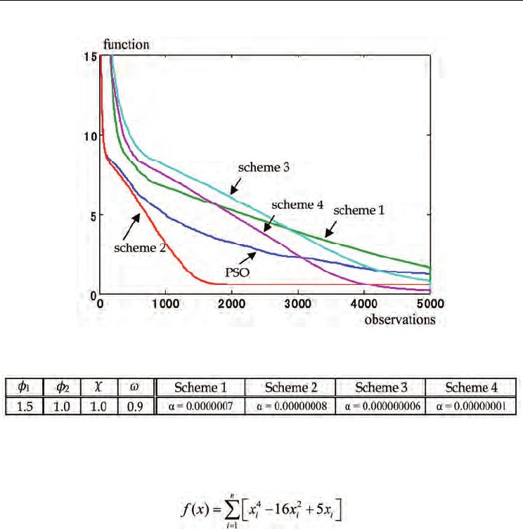
3. 2

-minima function

The 2

-minima function is

(8)

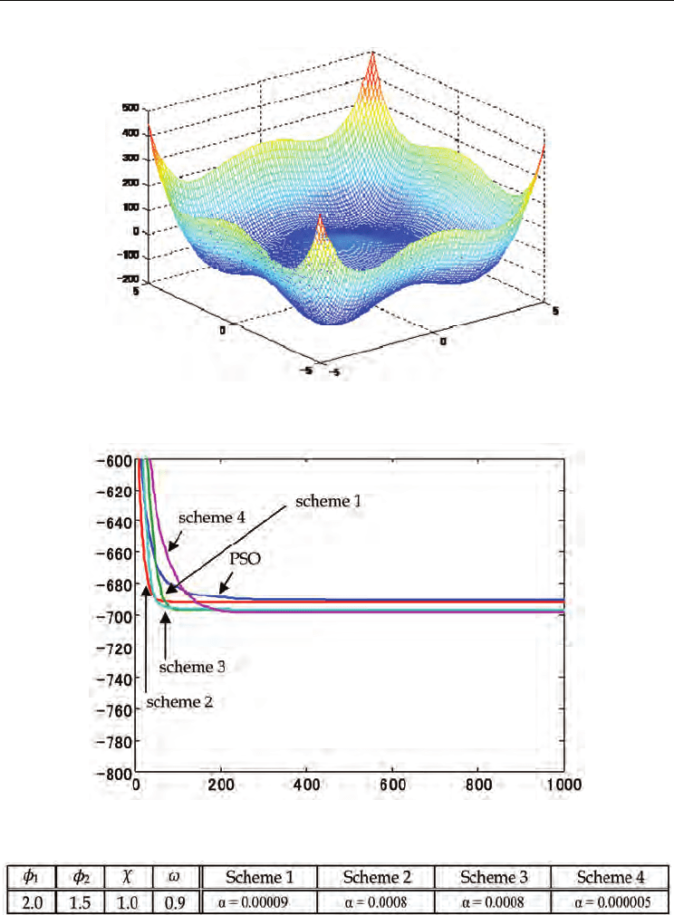
Shape of the function is shown in Fig.6. Searched area is -5 up to +5. Table 3 shows

parameters setting. The value of the global minimum of the function is -783.32.

The function has some local minimum points and relatively flat bottom. This deteriorates

search capability of the gradient method. Change of the best particle is also depicted in

Fig.7. The scheme 4 has relatively good performance for this case. The function has flat

bottom including a global minimum. In order to search the global minimum, it seems that

the swarm search is useful. Searching the global minimum using many particles is efficient.

Simultaneously, local search is necessary to find exact position of the global minimum. It

seems that the scheme 4 matched for the case.

As a result, we can say that the gradient search is important and combination with the

particle swarm optimization will give us a powerful tool.

Simultaneous Perturbation Particle Swarm Optimization and Its FPGA Implementation

355

Figure 6. 2

-minima function

Figure 7. Change of the best particle for 2

-minima function

Table 3. Parameters setting for 2

-minima function

Particle Swarm Optimization

356

5. FPGA implementation

Now, we implement the simultaneous perturbation particle swarm optimization using

FPGA. Then we can realize one feature of parallel operation of the particle swarm

optimization. This results in higher operation speed for optimization problems.

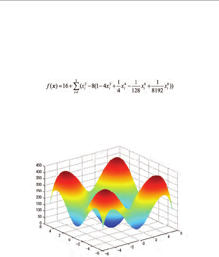
We adopted VHDL (VHSIC Hardware Description Language) in basic circuit design for

FPGA. The design result by VHDL is configured on MU200 - SX60 board with

EP1S60F1020C6 (Altera) (see Fig.8). This FPGA contains 57,120 LEs with 5,215,104 bit user

memory.

Figure 8. FPGA board MU200-SX60 (MMS)

Figure 9. Configuration of the SP particle swarm optimization system

Simultaneous Perturbation Particle Swarm Optimization and Its FPGA Implementation

357

Visual Elite (Summit) is used for the basic deign. Synplify Pro (Synplicity) carried out the

logical synthesis for the VHDL. QuartusII (Altera) is used for wiring.Overall system

configuration is shown in Fig.9. Basically, the system consists of three units; swarm unit,

detection unit and simultaneous perturbation unit.

In this system, we prepared three particles. These particles works parallel to obtain values of

a target function, and are updated their positions and velocity. Therefore, even if the system

has many particles, this does not effect on the overall operation speed. Number of the

particles in this system is restricted by the scale of target FPGA. We should economize the

design, if we would like to contain many particles.

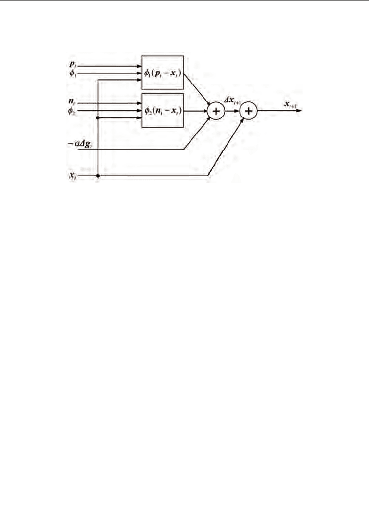
The target function with two parameters x

and x

is defined as follow;

(9)

Based on Rastrigin function, we assume this test function with optimal value of 0 and 8th

order. We would like to find the optimal point (0.0 0.0) in the range [-5.5 5.5]. Then optimal

value of the function is 0. Fig. 10 shows shape of the function.

Figure 10. Shape of the target function

5.1 Swarm unit

Swarm unit includes some particles which are candidate of the optimum point. Candidate

values are memorized and updated in these particle parts.

Configuration of the particle part is shown in Fig. 11. This part holds its position value and

velocity. At the same time, modifying quantities for all particles are sent by the

Particle Swarm Optimization

358

simultaneous perturbation unit. The particle part updates its position and velocity based on

these modifying quantities.

Figure 11. Particle part

5.2 Detection unit

The detection unit finds and holds the best estimated value for each particle. We refer this

estimator as individual best. And based on the individual best values of the each particle,

the unit searches the best one that all the particles have ever found. We call it the group best.

The individual best values and the group best value are stored in RAM. For iteration, new

positions for all particles are compared with corresponding values stored in RAM. If new

position is better, it is stored, that is, the individual best value is updated. Moreover, these

are used to determine the group best value.

These individual best values and the group best value are used in the swarm unit to update

the velocity.

5.3 Simultaneous perturbation unit

The simultaneous perturbation unit realizes calculation of evaluation function for each

particle, estimation of the gradient of the function based on the simultaneous perturbation.

As a result, the unit produces estimated gradient for all the particles. The results are sent to

the swarm unit.

5.4 Implementation result

Single precision floating point expression IEEE 574 is adopted to express all values in the

system. Ordinary floating point operations are used to realize the simultaneous perturbation

particle swarm optimization algorithm.

We searched the area of [-5.5 5.5]. Initial positions of the particles were determined

randomly from (2.401, 2.551), (-4.238, 4.026) or (-3.506, 1.753). Initial velocity was all zero.

Then we defined value of

is 1. Coefficients

and

in the algorithm were selected from

2i(=2), 2°(=1), 2-i(=0.5), 2-2(=0.25), 2-3(=0.125), 2-4(=0.0625), 2-5(=0.03125) or 2-6(=0.015625).

This simplifies multiplication of these coefficients. The multiplication can be carried out by

addition for exponent component.

Simultaneous Perturbation Particle Swarm Optimization and Its FPGA Implementation

359

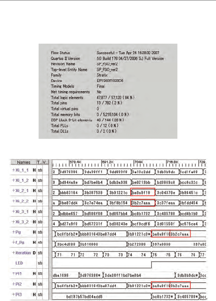
Design result is depicted in Fig.12. 84% of LE is used for all this system design. We should

economize the scale of the design, if we would like to implement much more particles in the

system. Or, we can also adopt time-sharing usage of the single particle part. Then total

operation speed will deteriorate.

Figure 12. Design result

Figure 13. Simulation result

Particle Swarm Optimization

360

Fig.13 shows a simulation result by Visual Elite. Upper six signals xi_l_l upto xi_3_2 denote

values of parameters x

and x

of three particles, respectively. Lower three signals HI upto

Pi3 are individual best values of three particles at the present iteration. x

and x

values are

consecutively memorized. Between these, the best one becomes group best shown in Pg

signal. f_Pg is the corresponding function value. In Fig.13 between three particle, the second

particle of Pi2 became the group best value of Pg. We can find END flag of "LED" at 75th

iteration.

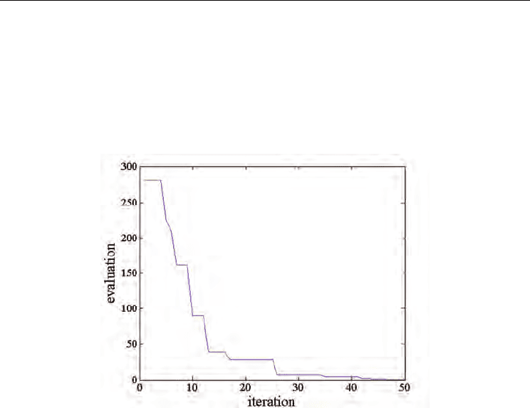
Figure 14. Operation result

Fig.14 shows a change of the evaluation function of the best of the swarm for iteration. The

system easily finds the optimum point with three particles. About 50 iteration, the best

particle is very close to global optimum. As mentioned before, after 75 iteration, the system

stoped with an end condition.

6. Conclusion

In this paper, we presented hardware implementation of the particle swarm optimization

algorithm which is combination of the ordinary particle swarm optimization and the

simultaneous perturbation method. FPGA is used to realize the system. This algorithm

utilizes local information of objective function effectively without lack of advantage of the

original particle swarm optimization. Moreover, the FPGA implementation gives higher

operation speed effectively using parallelism of the particle swarm optimization. We

confirmed viability of the system.

7. Acknowledgement

This work is financially supported by Grant-in-Aid for Scientific Research (No.19500198) of

the Ministry of Education, Culture, Sports, Science and Technology (MEXT) of Japan, and

the Intelligence system technology and kansei information processing research group,