Lazinica A. (ed.) Particle Swarm Optimization
Подождите немного. Документ загружается.

Particle Swarm Optimization for HW/SW Partitioning
61
0 100 200 300 400 500 600 700 800 900 1000
-30
-20
-10
0
10
20
30
40
50
60
70
Design Size in Nodes
Speed Improvement
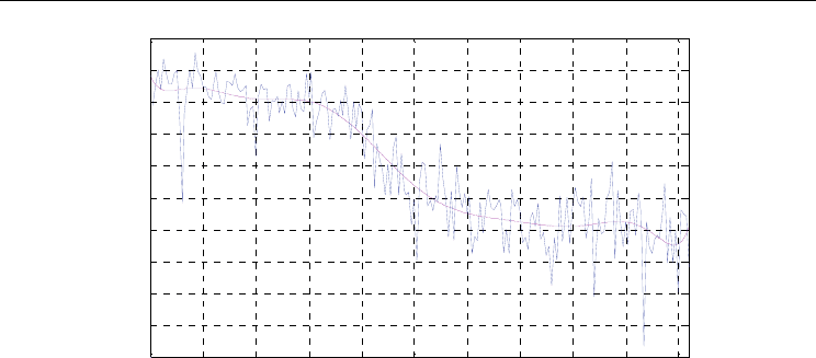
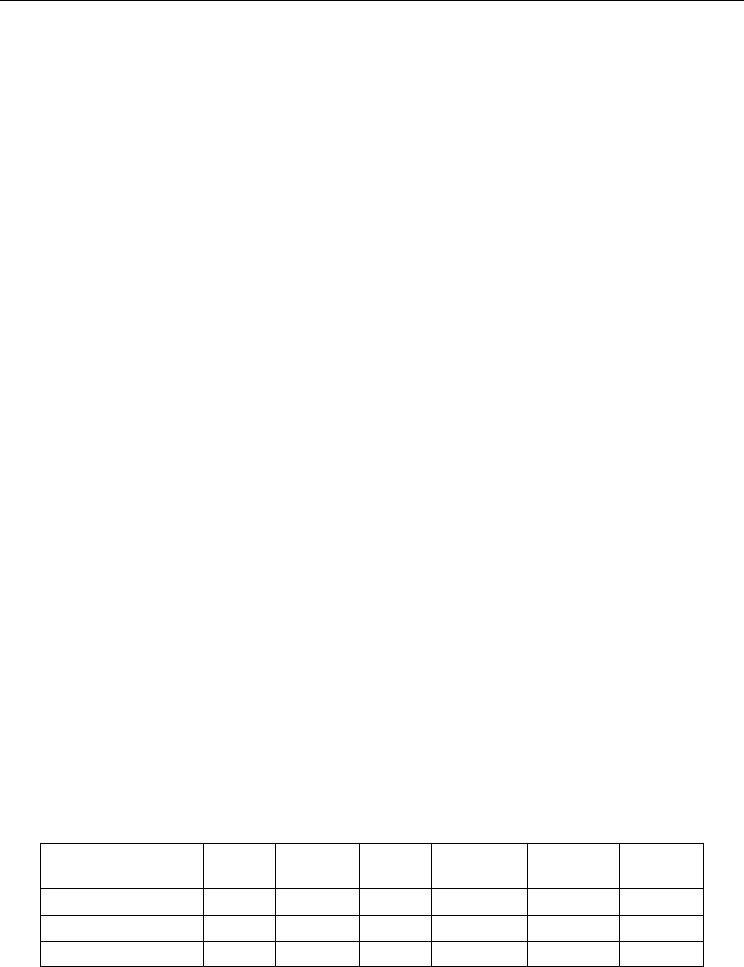
Figure 8. Speed improvement
Fig. 8 represents the performance (speed) improvement of PSO over GA (original and fitted
curve, the curve fitting is done using MATLAB Basic Fitting tool). Re-excited PSO is not
included as it depends on multi-round scheme where it starts a new round internally when
the previous round terminates, while GA and PSO runs once and produces their outputs
when a termination criterion is met.
It is noticed that in a few number of points in Fig. 8, the speed improvement is negative
which means that GA finishes before PSO, but the design quality in Fig. 7 does not show
any negative values. Fig. 7 also shows that, on the average, PSO outperforms GA by a ratio
of 7.8% improvements in the result quality and Fig. 8 shows that, on the average, PSO
outperforms GA by a ratio 29.3% improvement in speed.
On the other hand, re-excited PSO outperforms GA by an average ratio of 17.4% in design
quality, and outperforms normal PSO by an average ratio of 10.5% in design quality.
Moreover, Fig. 8 could be divided into three regions. The first region is the small size
designs region (lower than 400 nodes) where the speed improvement is large (from 40% to
60%). The medium size design region (from 400 to 600 nodes) depicts an almost linear
decrease in the speed improvement from 40% to 10%. The large size design region (bigger
than 600 nodes) shows an almost constant (around 10%) speed improvement, with some
cases where GA is faster than PSO. Note that most of the practical real life HW/SW
partitioning problems belong to the first region where the number of nodes < 400.
3.6 Constrained Problem Formulation
3.6.1 Constraints definition and violation handling
In embedded systems, the constraints play an important role in the success of a design, where
hard constraints mean higher design effort and therefore a high need for automated tools to
guide the designer in critical design decisions. In most of the cases, the constraints are mainly the
software deadline times (for real-time systems) and the maximum available area for hardware.
For simplicity, we will refer to them as software constraint and hardware constraint respectively.
Mann [2004] divided the HW/SW partitioning problem into 5 sub-problems (P
1
– P
5
). The
unconstrained problem (P
5
) is discussed in Section 3.3. The P
1
problem involves with both
Particle Swarm Optimization
62
Hardware and Software constraints. The P
2
(P
3
) problem deals with hardware (software)
constrained designs. Finally, the P
4
problem minimizes HW/SW communications cost while
satisfying hardware and software constraints. The constraints affect directly the cost
function. Hence, equation (3) should be modified to account for constraints violations.
In Lopez-Vallejo et al. [2003] three different techniques are suggested for the cost function
correction and evaluation:
Mean Square Error minimization: This technique is useful for forcing the solution to meet
certain equality, rather than inequality, constraints. The general expression for Mean Square
Error based cost function is:
2
i
2
ii
ii
constraint
)constraint(cost
*k MSE_cost
−
=
(4)
where constraint
i
is the constraint on parameter i and k
i
is a weighting factor. The cost
i
is the
parameter cost function. cost
i
is calculated using the associated term (i.e. area or delay) of
the general cost function (3).
Penalty Methods: These methods punish the solutions that produce medium or large
constraints violations, but allow invalid solutions close to the boundaries defined by the
constraints to be considered as good solutions [Lopez-Vallejo et al. 2003]. The cost function
in this case is formulated as:
∑∑
+=
ici
ci
i
i
i
)x,ci(viol*k
tcosTotal
)x(tcos
*k)x(Cost
(5)
where x is the solution vector to be evaluated, k
i
and k
ci
are weighting factors (100 in our
case). i denotes the design parameters such as: area, delay, power consumption, etc., ci
denotes a constrained parameter, and viol(ci,x) is the correction function of the constrained
parameters. viol(ci,x) could be expressed in terms of the percentage of violation defined by :
⎪
⎪
⎩
⎪
⎪
⎨
⎧
>
−
<
=
)ciint(constra)x(tcos
(ci)constraint
(ci)constraint)x(tcos
)ciint(constra)x(tcos0
x)viol(ci,
i
i
i
(6)
Lopez-Vallejo and Lopez et al. [2003] proposed to use the squared value of viol(ci,x).
The penalty methods have an important characteristic in which there might be invalid
solutions with better overall cost than valid ones. In other words, the invalid solutions are
penalized but could be ranked better than valid ones.
Barrier Techniques: These methods forbid the exploration of solutions outside the allowed
design-space. The barrier techniques rank the invalid solutions worse than the valid ones.
There are two common forms of the barrier techniques. The first form assigns a constant
high cost to all invalid solutions (for example infinity). This form is unable to differentiate
between near-barrier or far-barrier invalid solutions. it also needs to be initialized with at
least one valid solution, otherwise all the costs are the same (i.e. ∞) and the algorithm fails.
The other form, suggested in Mann [2004], assigns a constant-base barrier to all invalid
solutions. This base barrier could be a constant larger than maximum cost produced by any
valid solution. In our case for example, from equation (3), each cost term is normalized such
that its maximum value is one. Therefore, a good choice of the constant-base penalty is "one"
for each violation ("one" for hardware violation, "one" for software violation, and so on).
Particle Swarm Optimization for HW/SW Partitioning
63
3.6.2 Constraints modeling
In order to determine the best method to be adopted, a comparison between the penalty
methods (first order or second order percentage violation term) and the barrier methods
(infinity vs. constant-base barrier) is performed. The details of the experiments are not
shown here for the sake of brevity.
Our experiments showed that combining the constant-base barrier method with any penalty
method (first-order error or second-order error term) gives higher quality solutions and
guarantees that no invalid solutions beat valid ones. Hence, in the following experiments,
equation (7) will be used as the cost function form. Our experiments further indicate that the
second-order error penalty method gives a slight improvement over first-order one.
For double constraints problem (P
1
), generating valid initial solutions is hard and time
consuming, and hence, the barrier methods should be ruled out for such problems. When
dealing with single constraint problems (P
2
and P
3
), one can use the Fast Greedy Algorithm
(FGA) proposed by Mann [2004] to generate valid initial solutions. FGA starts by assigning
all nodes to the unconstrained side. It then proceeds by randomly moving nodes to the
constrained side until the constraint is violated.
))ci(viol_Barrier)x,ci(viol_Penalty(k
tcosTotal
)x(tcos
*k)x(Cost
ici
ci
i
i
i
++=
∑∑
(7)
3.6.3 Single constraint experiments
As P
2
and P
3
are treated the same in our formulation, we consider the software constrained
problem (P
3
) only. Two experiments were performed, the first one with relaxed constraint
where the deadline (Maximum delay) is 40% of all-Software solution delay, the second one
is a hard real-time system where the deadline is 15% of the all-Software solution delay. The
parameters used are the same as in Section 3.4. Fast Greedy Algorithm is used to generate
the initial solutions and re-excited PSO is performed for 10 rounds. In the cases of GA and
normal PSO only, all results are based on averaging the results of 100 runs.
For the first experiment; the average quality of the GA is ~ 137.6 while for PSO it is ~ 131.3,
and for re-excited PSO it is ~ 120. All final solutions are valid due to the initialization
scheme used (Fast Greedy Algorithm).
For the second experiment, the average quality of the solution of GA is ~ 147 while for PSO
it is ~ 137 and for re-excited PSO it is ~ 129.
The results confirm our earlier conclusion that the re-excited PSO again outperforms normal
PSO and GA, and that the normal PSO again outperforms GA.
3.6.4 Double constraints experiments
When testing P
1
problems, the same parameters as the single-constrained case are used
except that FGA is not used for initialization. Two experiments were performed: balanced
constraints where maximum allowable hardware area is 45% of the area of the all-Hardware
solution and the maximum allowable software delay is 45% of the delay of the all-Software
solution. The other one is an unbalanced-constraints problem where maximum allowable
hardware area is 60% of area of the all-Hardware solution and the maximum allowable
software delay is 20% of the delay of the all-Software solution. Note that these constraints
are used to guarantee that at least a valid solution exists.
Particle Swarm Optimization
64
For the first experiment, the average quality of the solution of GA is ~ 158 and invalid
solutions are obtained during the first 22 runs out of xx total runs. The best valid solution
cost was 137. For PSO the average quality is ~ 131 with valid solutions during all the runs.
The best valid solution cost was 128.6. Finally for the re-excited PSO; the final solution
quality is 119.5. It is clear that re-excited PSO again outperforms both PSO and GA.
For the second experiment; the average quality of the solution of GA is ~ 287 and no valid
solution is obtained during the runs. Note that a constant penalty barrier of value 100 is
added to the cost function in the case of a violation. For PSO the average quality is ~ 251 and
no valid solution is obtained during the runs. Finally, for the re-excited PSO, the final
solution quality is 125 (As valid solution is found in the seventh round). This shows the
performance improvement of re-excited PSO over both PSO and GA.
Hence, for the rest of this Chapter, we will use the terms PSO and re-excited PSO
interchangeably to refer to the re-excited algorithm.
3.7 Real-Life Case Study
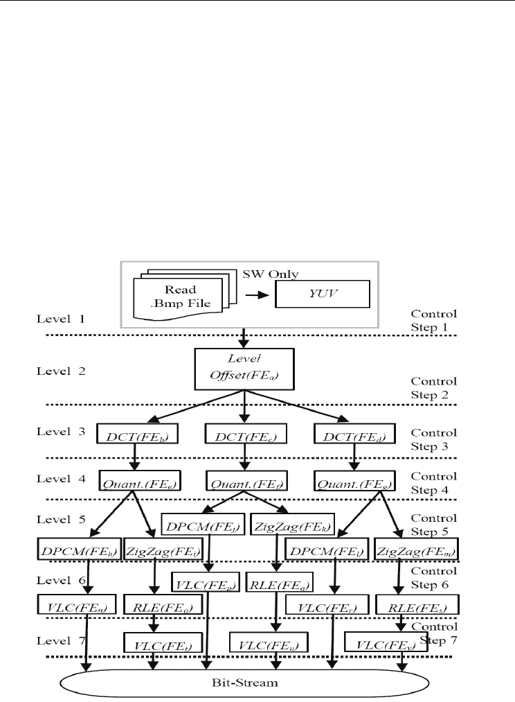
Figure 9. CDFG for JPEG encoding system [Lee et al. 2007c]
Particle Swarm Optimization for HW/SW Partitioning
65
To further validate the potential of PSO algorithm for HW/SW partitioning problem we
need to test it on a real-life case study, with a realistic cost function terrain. We also wanted
to verify our PSO generated solutions against a published “benchmark” design. The
HW/SW cost matrix for all the modules of such real life case study should be known. We
carried out a comprehensive literature search in search for such case study. Lee et al. [2007c]
provided such details for a case study of the well-known Joint Picture Expert Group (JPEG)
encoder system. The hardware implementation is written in "Verilog" description language,
while the software is written in "C" language. The Control-Data Flow Graph (CDFG) for this
implementation is shown in Fig. 9. The authors pre-assumed that the RGB to YUV converter
is implemented in SW and will not be subjected to the partitioning process. For more details
regarding JPEG systems, interested readers can refer to Jonsson [2005].
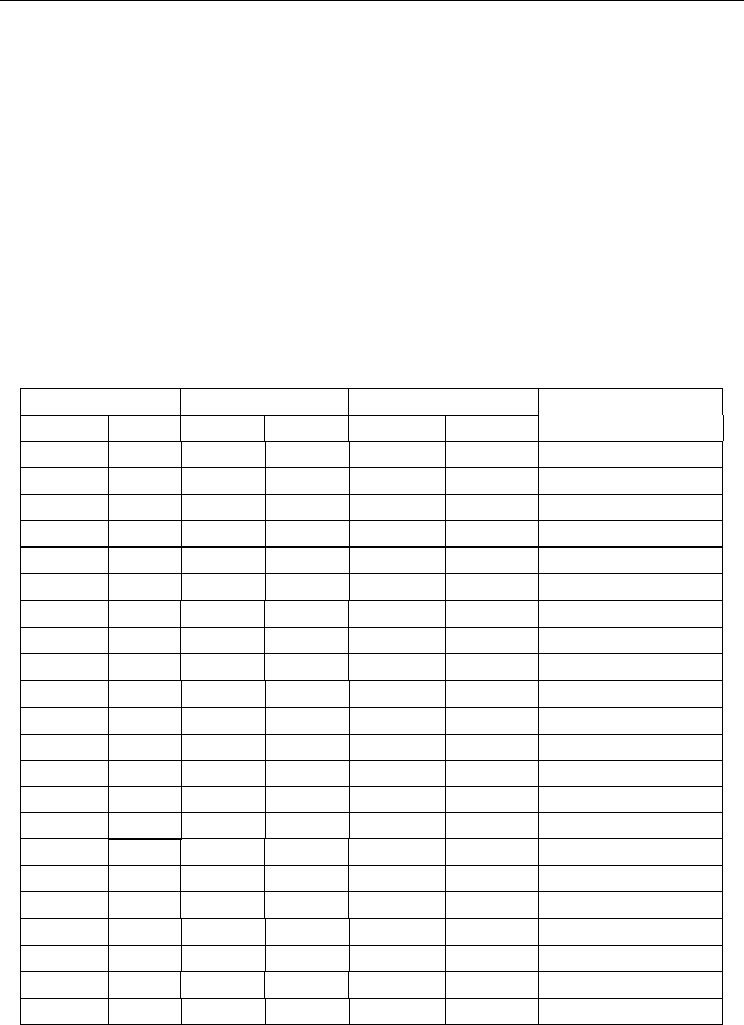
Table 1 shows measured data for the considered cost metrics of the system components.
Including such table in Lee et al. [2007c] allows us to compare directly our PSO search
algorithm with the published ones without re-estimating the HW or SW costs of the design
modules on our platform. Also, armed with this data, there is no need to re-implement the
published algorithms or trying to obtain them from their authors.
Execution Time Cost Percentage Power Consumption Component
HW(ns) SW(us) HW(10
-3
) SW(10
-3
) HW(mw) SW(mw)
155.264 9.38 7.31 0.58 4 0.096
Level Offset (FE
a
)
1844.822 20000 378 2.88 274 45
DCT (FE
b
)
1844.822 20000 378 2.88 274 45
DCT (FE
c
)
1844.822 20000 378 2.88 274 45
DCT (FE
d
)
3512.32 34.7 11 1.93 3 0.26
Quant (FE
e
)
3512.32 33.44 9.64 1.93 3 0.27
Quant (FE
f
)
3512.32 33.44 9.64 1.93 3 0.27
Quant (FE
g
)
5.334 0.94 2.191 0.677 15 0.957
DPCM (FE
h
)
399.104 13.12 35 0.911 61 0.069
ZigZag (FE
i
)
5.334 0.94 2.191 0.677 15 0.957
DPCM(FE
j
)
399.104 13.12 35 0.911 61 0.069
ZigZag (FE
k
)
5.334 0.94 2.191 0.677 15 0.957
DPCM (FE
l
)
399.104 13.12 35 0.911 61 0.069
ZigZag (FE
m
)
2054.748 2.8 7.74 14.4 5 0.321
VLC (FE
n
)
1148.538 43.12 2.56 6.034 3 0.021
RLE (FE
o
)
2197.632 2.8 8.62 14.4 5 0.321
VLC (FE
p
)
1148.538 43.12 2.56 6.034 3 0.021
RLE (FE
q
)
2197.632 2.8 8.62 14.4 5 0.321
VLC (FE
r
)
1148.538 43.12 2.56 6.034 3 0.021
RLE (FE
s
)
2668.288 51.26 19.21 16.7 6 0.018
VLC (FE
t
)
2668.288 50 1.91 16.7 6 0.018
VLC (FE
u
)
2668.288 50 1.91 16.7 6 0.018
VLC (FE
v
)
Table 1. Measured data for JPEG system
Particle Swarm Optimization
66
The data is obtained through implementing the hardware components targeting ML310
board using Xilinx ISE 7.1i design platform. Xilinx Embedded Design Kit (EDK 7.1i) is used
to measure the software implementation costs.
The target board (ML310) contains Virtex2-Pro XC2vP30FF896 FPGA device that contains
13696 programmable logic slices and 2448 Kbytes memory and two embedded IBM Power
PC (PPC) processor cores. In general, one slice approximately represents two 4-input Look-
Up Tables (LUTs) and two Flip-Flops [Xilinx 2007].
The first column in the table shows the component name (cf. Fig. 9) along with a character
unique to each component. The second and third columns show the power consumption in
mWatts for the hardware and software implementations respectively. The fourth column
shows the software cost in terms of memory usage percentage while the fifth column shows
the hardware cost in terms of slices percentage. The last two columns show the execution
time of the hardware and software implementations.
Lee et al. [2007c] also provided detailed comparison of their methodology with another four
approaches. The main problem is that the target architecture in Lee et al. [2007c] has two
processors and allows multi-processor partitioning while our target architecture is based on
a single processor. A slight modification in our cost function is performed that allows up to
two processors to run on the software part concurrently.
Equation (3) is used to model the cost function after adding the memory cost term as shown
in Equation (8)
⎭
⎬
⎫
⎩
⎨
⎧
η+γ+β+α=
tcosallMEM
tcosMEM
tcosallPOWER
tcosPOWER
tcosallSW
tcosSW
tcosallHW
tcosHW
*100Cost
(8)
The added memory cost term (MEMcost) and its weight factor (η) account for the memory
size (in bits). allMEMcost is the maximum size (upper-bound) of memory bits i.e., memory
size of all software solution.
Another modification to the cost function of Equation (8) is affected if the number of
multiprocessors is limited. Consider that we have only two processors. Thus, only two
modules can be assigned to the SW side at any control step. For example, in the step 3 of Fig.
9, no more than two DCT modules can be assigned to the SW side. The solution that assigns
the three DCT modules of this step to SW side is penalized by a barrier violation term of
value "one".
Finally, as more than one hardware component could run in parallel, the hardware delay is
not additive. Hence, we calculate the hardware delay by accumulation the maximum delay
of each control steps as shown in Fig. 9. In other words, we calculate the critical-path delay.
In Lee et al. [2007c], the results of four different algorithms were presented. However, for
the sake brevity, details of such algorithms are beyond the scope of this chapter. We used
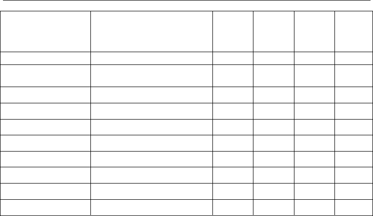
these results and compared them with our algorithm in Table 2.
In our experiments, the parameters used for the PSO are the population size is fixed to 50
particles, the round terminates after 50 unimproved runs, and 100 runs must run at the
beginning to avoid trapping in local minimum. The number of re-excited PSO rounds is
selected by the user.
The power constraint is constrained to 600 mW, area and memory are constrained to the
maximum available FPGA resources, i.e. 100%, and maximum number of concurrent
software tasks is two.
Particle Swarm Optimization for HW/SW Partitioning
67
Method
Results
Lev / DCT / Q / DPCM-Zig /
VLC-RLE / VLC
Execution
Time (us)
Memory
(KB)
Slice use
rate (%)
Power
(mW)
FBP [Lee et al. 2007c] 1/001/111/101111/111101/111 20022.26 51.58 53.9 581.39
GHO [Lee et al.
2007b]
1/010/111/111110/111111/111
20021.66 16.507
54.7 586.069
GA [Lin et al. 2006] 0/010/010/101110/110111/010 20111.26 146.509 47.1 499.121
HOP [Lee et al. 2007a] 0/100/010/101110/110111/010 20066.64 129.68 56.6 599.67
PSO-delay 1/010/111/111110/111111/111
20021.66 16.507
54.7 586.069
PSO-area 0/100/001/111010/110101/010 20111.26 181.6955
44.7 494.442
PSO-power 0/100/001/111010/110101/010 20111.26 181.6955
44.7 494.442
PSO-memory 1/010/111/111110/111111/111
20021. 66 16.507
54.7 586.069
PSO-NoProc 0/000/111/000000/111111/111 20030.9 34.2328 8.6 189.174
PSO-Norm 0/010/111/101110/111111/111 20030.9 19.98 50.6 521.234
Table 2. Comparison of partitioning results
Different configurations of the cost function are tested for different optimization goals. PSO-
delay, PSO-area, PSO-power, and PSO-memory represent the case where the cost function
includes only one term, i.e. delay, area, power, and memory, respectively. PSO-NoProc is
the normal PSO-based algorithm with the cost function shown in equation (7) but the
number of processors is unconstrained. Finally, PSO-Norm is the normal PSO with all
constraints being considered, i.e. the same as PSO-NoProc with maximum number of two
processors.
The second column in Table 2 shows the resulting partition where '0' represents software
and '1' represents hardware. The vector is divided into sets, each set represents a control
step as shown in Fig. 9. The third to fifth columns of this table list the execution time,
memory size, % of slices used and the power consumption respectively of the optimum
solutions obtained according to the algorithms identified in the first column. As shown in
the table, the bold results are the best results obtained for each design metrics.
Regarding PSO performance, all the PSO-based results are found within two or three rounds
of the Re-excited PSO. Moreover, for each individual optimization objective, PSO obtains the
best result for that specific objective. For example, PSO-delay obtains the same results as
GHO algorithm [ref.] does and it outperforms the other solutions in the execution time and
memory utilization and it produces good quality results that meet the constraints. Hence,
our cost function formulation enables us to easily select the optimization criterion that suits
our design goals.
In addition, PSO-a and PSO-p give the same results as they try to move nodes to software
while meeting the power and number of processors constraints. On the other hand, PSO-del
and PSO-mem try to move nodes to hardware to reduce the memory usage and the delay,
so their results are similar.
PSO-NoProc is used as a what-if analysis tool, as its results answer the question of what is
the optimum number of parallel processors that could be used to find the optimum design.

Particle Swarm Optimization
68
In our case, obtaining six processors would yield the results shown in the table even if three
of them will be used only for one task, namely, the DCT.
4. Extensions
4.1 Modeling Hardware Implementation alternatives
As shown previously, HW/SW partitioning depends on the HW area, delay, and power
costs of the individual nodes. Each node represents a grain (from an instruction up to a
procedure), and the grain level is selected by the designer. The initial design is usually
mapped into a sequencing graph that describes the flow dependencies of the individual
nodes. These dependencies limit the maximum degree of parallelism possible between these
nodes. Whereas a sequencing graph denotes the partial order of the operations to be
performed, the scheduling of a sequencing graph determines the detailed starting time for
each operation. Hence, the scheduling task sets the actual degree of concurrency of the
operations, with the attendant delay and area costs [De Micheli 1994]. In short, delay and
area costs needed for the HW/SW partitioning task are only known accurately post the
scheduling task. Obviously, this situation calls for time-wasteful iterations. The other
solution is to prepare a library of many implementations for each node and select one of
them during the HW/SW partitioning task as the work done by Kalavade and Lee [2002].
Again, such approach implies a high design time cost.
Our approach to solve this egg-chicken
coupling between the partitioning and scheduling
tasks is as follows: represent the hardware solution of each node by two limiting solutions,
HW
1
and HW
2
, which are automatically generated from the functional specifications. These
two limiting solutions bound the range of all other possible schedules. The partitioning
algorithm is then called on to select the best implementation for the individual nodes: SW,
HW
1
or HW
2
. These two limiting solutions are:
1. Minimum-Latency solution: where As-Soon-As-Possible (ASAP) scheduling algorithm
is applied to find the fastest implementation by allowing unconstrained concurrency.
This solution allows for two alternative implementations, the first where maximum
resource-sharing is allowed. In this implementation, similar operational units are
assigned to the same operation instance whenever data precedence constraints allow.
The other solution, the non-shared parallel solution, forbids resource-sharing altogether
by instantiating a new operational unit for each operation. Which of these two parallel
solutions yields a lower area is difficult to predict as the multiplexer cost of the shared
parallel solution, added to control the access to the shared instances, can offset the extra
area cost of the non-shared solution. Our modeling technique selects the solution with
the lower area. This solution is, henceforth, referred to as the parallel hardware
solution.
2. Maximum Latency solution: where no concurrency is allowed, or all operations are
simply serialized. This solution results in the maximum hardware latency and the
instantiation of only one operational instance for each operation unit. This solution is,
henceforth, referred to as the serial hardware solution.
To illustrate our idea, consider a node that represents the operation y = (a*b) + (c*d). Fig.
10.a (10.b) shows the parallel (serial) hardware implementations.
From Fig. 10 and assuming that each operation takes only one clock cycle, the first
implementation finishes in 2 clock cycles but needs 2 multiplier units and one adder unit.
The second implementation ends in 3 clock cycles but needs only one unit for each operation
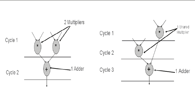
Particle Swarm Optimization for HW/SW Partitioning
69
(one adder unit and one multiplier unit). The bold horizontal lines drawn in Fig. 10
represent the clock boundaries.
(a) (b)
Figure 10. Two extreme implementations of y = (a*b) + (c*d)
In general, the parallel and serial HW solutions have different area and delay costs. For
special nodes, these two solutions may have the same area cost, the same delay cost or the
same delay and area costs. The reader is referred to Abdelhalim and Habib [2007] for more
details on such special nodes.
The use of two alternative HW solutions converts the HW/SW optimization problem from a
binary form to a tri-state form. The effectiveness of the PSO algorithm for handling this
extended HW/SW partitioning problem is detailed in Section 4.3.
4.2 Communications Cost Modeling
The Communications cost term in the context of HW/SW partitioning represents the cost
incurred due to the data and control passing from one node to another in the graph
representation of the design. Earlier co-design approaches tend to ignore the effect of
HW/SW communications. However, many recent embedded systems are communications
oriented due to the heavy amount of data to be transferred between system components.
The communications cost should be considered at the early design stages to provide high
quality as well as feasible solutions. The communication cost can be ignored if it is between
two nodes on the same side (i.e., two hardware nodes or two software nodes). However, if
the two nodes lie on different sides; the communication cost cannot be ignored as it affects
the partitioning decisions. Therefore, as communications are based on physical channels, the
nature of the channel determines the communication type (class). In general, the HW/SW
communications between the can be classified into four classes [Ernest 1997]:
1. Point-to-point communications
2. Bus-based communications
3. Shared memory communications
4. Network-based communications
To model the communications cost, a communication class must be selected according to the
target architecture. In general, the model should include one or more of the following cost
terms [Luthra et al. 2003]:
1. Hardware cost: The area needed to implement the HW/SW interface and associated
data transfer delay on the hardware side.
Particle Swarm Optimization
70
2. Software cost: The delay of the software interface driver on the software side.
3. Memory size: The size of the dedicated memory and registers for control and data
transfers as well as shared memory size.
The terms could be easily modeled within the overall delay, hardware area and memory
costs of the system, as shown in equation (8).
4.3 Extended algorithm experiments
As described in Section 3.3, the input to the algorithm is a graph that consists of a number of
nodes and number of edges. Each node (edge) is associated with cost parameters. The used
cost parameters are:
Serial hardware implementation cost: which is the cost of implementing the node in
serialized hardware. The cost includes HW area as well as the associated latency (in clock
cycles).
Parallel hardware implementation cost: which is the cost of implementing the node in
parallel hardware. The cost includes HW area as well as the associated latency (in clock
cycles).
Software implementation cost: the cost of implementing the node in software (e.g.
execution clock cycles and the CPU area).
Communication cost: the cost of the edge if it crosses the boundary between the HW and
the SW sides (interface area and delay, SW driver delay and shared memory size).
For experimental purposes, these parameters are randomly generated after considering the
characteristics of each parameter, i.e. Serial HW area ≤ Parallel HW area, and
SW delay ≤ Serial HW delay ≤ Parallel HW delay.
The needed modification is to allow each node in the PSO solution vector to have three
values: “0” for software, “1” for serial hardware and “2” for parallel hardware.
The parameters used in the implementation are: No. of particles (Population size) n = 50,
No. of design size (m) = 100 nodes, No. of communication edges (e) = 200, No. The number
of re-exited PSO rounds set to a predefined value = 50. All other parameters are taken from
Section 3.4. The constraints are: Maximum hardware area is 65% of the all-Hardware
solution area, and the maximum delay is 25% of the all-Software solution delay.
4.3.1 Results
Three experiments were performed. The first (second) experiment uses the normal PSO with
only the serial (parallel) hardware implementation. The third experiment examines the
proposed tristate formulation where the hardware is represented by two solutions (serial
and parallel solutions). The results are shown in Table 3.
Area
Cost
Delay
Cost
Comm.
Cost
Serial HW
nodes
Parallel
HW nodes
SW
nodes
Serial HW
34.9%
30.52%
1.43% 99 N/A 1
Parallel HW
57.8%
29.16%
32.88% N/A 69 31
Tri-state formul.
50.64% 23.65% 18.7% 31 55 14
Table 3. Cost result of different hardware alternatives schemes
As shown in this table, the serial hardware solution pushes approximately all nodes to
hardware (99 out of 100) but fails to meet the deadline constraint due to the relatively large