Lewis R.I. Turbomachinery Performance Analysis
Подождите немного. Документ загружается.

114
Simplified meridional flow analysis for axial turbomachines
An equivalent equation for compressible flow can be developed by making use of
the following thermodynamic relationship which links temperature T, specific entropy
s and specific enthalpy h to p and p:
T ds = dh -1 dp
P
= dho- ldpo
P
(5.15)
where the stagnation enthalpy is defined as ho = h + c2/2. Dividing throughout by
dr and substituting for
(1/p)(dpo/dr)
in Eqn (5.14), we have finally the
radial
equilibrium equation for compressible flow:
The axial velocity
Cx
is thus a function of the radial distribution not only of
rco
but
also of ho and s.
5,3
Solution of the radial equilibrium equation for the
inverse and direct problems
Two types of problem may be identified as follows:
(1)
(2)
The 'Inverse' or 'Design' problem.
In the design sequence outlined in Section
5.1, once the velocity triangles have been selected ho and
co
are known at all
radii as part of the design specification. The radial distribution of specific
entropy s may also be obtained from a first estimate of the losses or r/x-r
from model test data. Solution of the radial equilibrium Eqn (5.16) then
yields a new estimate of the axial velocity distribution
Cx
and hence an
updating of the velocity triangles and thus flow angles prior to blade profile
selection. This is the
design problem.
The 'Direct' or 'Analysis' problem.
We may postulate the opposite problem
in which we are presented with an existing turbomachine of known blade
geometry and asked to predict its fluid dynamic performance. This is the
analysis problem.
Theoretical analysis to deal with these two rather different problems will now be
presented with the help of numerical examples in Sections 5.3.1 and 5.3.2.
5.3.1 Solution of the inverse radial equilibrium problem
This is best illustrated by considering the case of a set of inlet guide vanes which
are to be designed to generate a solid body swirling flow.
Example 5.2 'Solid body' swirl inlet guide vanes
Consider the case of flow through an inlet guide vane blade row, Fig. 5.3(a). In this
case the swirl velocity
co
is to be proportional to radius at station 3 a long way
downstream of the blade row. We shall also assume that ho and s are both constant
5.3 Solution of the radial equilibrium equation 115
throughout the flow regime, namely
co = kr (where k is a constant)
ho = constant
s = constant
Problem
Derive an analytical solution for Cx as a function of r.
(5.17)
Solution
In view of Eqns (5.17b) and (5.17c), the radial equilibrium Eqn (5.16) reduces to
dcx co d(rco)
0 = Cx ~ ~ (5.16a)
r dr
which may be rewritten
dc 2 2co d(rco)
dr r dr
and hence, after integration, at radius r we have
Cx(r) = K1- 2 --d(rco)
r
(5.18)
Introduction of Eqn (5.17a) for the solid body rotation case then results in
Cx = N/K1 - 2k 2 r 2
= V'K 1 - 2r 2
(5.19)
The constant of integration K 1 can be evaluated by application of the mass
flow continuity equation. Thus the mass flow rh through the annulus may be
expressed as
in = pCx 2 7rr dr = pCx 2 zrr dr
station 1 - (entry) station 3 - (exit)
(5.20)
where Cx is the mean axial velocity and thus Cx = Cx at entry to the annulus. Assuming
incompressible flow and introducing Eqn (5.19), Eqn (5.20) becomes
Cx(r 2 - r2h) = 2 rV'K1- 2k2r 2 dr
1
= 3--~ [(K1- 2k2r2)3/2 _ (g 1 - 2kir2) 312]
(5.21)
Because of the complexity of Eqn (5.21), K1 cannot be evaluated explicitly and can
only be derived by successive approximations. Nevertheless a reasonable approximate
analytical solution may be derived as follows.
116 Simplified meridional flow analysis for axial turbomachines
Approximate solution matching Cx at the root mean square radius
rms
= 1 2 r 2) ThusEqn
Let us assume that
Cx = Cx
at the r.m.s, radius, namely
rms V'~(r h + .
(5.19) yields directly an estimate for K1, namely
K 1 = C 2 + 2(Corms) 2
= C 2 + 2c2~(rms/rt) 2
= C 2 + c2~(1 + h 2)
(5.22)
Thus finally, at other radii r, from Eqn (5.18) we have
cx
]
Cx
~ (5.23)
Numerical solution of the inverse problem
A much more flexible approach applicable to any radial distribution of
co
is to
evaluate Eqns (5.18) and (5.20) numerically. First let us define the function
f(r) = 2 frh" COr d(rco)
(5.24)
so that Eqn (5.18) becomes
Cx(r) = X/K 1 - f(r)
(5.25)
From the continuity equation (5.20) we may define a mass flow function
rh
S=m
2~rp
Cx (r 2 _ r2 )
=-~
= s rt
r~/K1 _ f(r) dr
h
at -~ upstream of blade row
J
at +~ downstream of blade row
(5.26)
For numerical analysis, the annulus may be represented by m radial steps between
hub and tip radii
r h
and rt of thickness Ar= (rt-rh)/m.
f(r)
may then be
approximated at radius
rj
by
J
f (rj) = 2 E
cOm''''~i (ri+ 1 Coi+ 1 -- ricoi)
(5.27)
i=1
rmi
_.1
where
rmi = 89 i + ri+
1) and
Com i ~(coi+ 1 + coi).
The mass function S may then also
be evaluated numerically if Eqn (5.26) is rewritten
In
S 1 --
Ar E
rmi~//K1-f(ri)
(5.28)
i=1
5.3 Solution of the radial equilibrium equation
117
Since the constant K1 is initially of unknown value, a method of successive
approximations will be required. The technique adopted in the Pascal program
RE-DES, provided on the accompanying PC disc, follows that of Newton. As a first
estimate the value of K1 given by the approximate analytical method of Eqn (5.22)
may be used to begin the process. We may then evaluate Sa and also the nearby value
$2 given by
m
$2 = Ar E
rmi~//gl -t- AK 1 - f(ri)
(5.29)
i=1
where
AK 1
is a small increment in
K 1 (e.g.
AK1/K 1
=
0.01). A revised estimate of
K1
then follows by extrapolation from
-s1
(K1)revise d=K I+AK 1 $2_S 1
(5.30)
Application of this procedure to a solid body swirl with mean axial velocity
Cx
= 1.0
and tip swirl velocity
co
= 1.0 produces the solution shown in Table 5.3, which shows
the precise prediction from computer program RE-DES compared with the
approximate analytical solution of Eqn (5.23). To achieve numerical accuracy it is
necessary to interpolate the initial
(r, co)
data to provide many more radial steps. A
Lagrangian interpolation procedure is included in RE-DES and for the above
computations m = 400 radial divisions of the annulus were used.
Results for two other vortex flows have also been calculated using RE-DES and
these are shown in Table 5.4. Let us now consider these in turn.
Example 5.3 Free-vortex flow
Since the function
f(r),
Eqn (5.24), is zero for this case, the axial velocity must be
uniform and equal to the mean velocity
Cx.
This is borne out by the numerical
prediction as can be seen from Table 5.4.
Example 5.4 Constant swirl velocity
c o
Problem
Following the lines of the analysis given in Example 5.2 for solid body flow, the reader
is invited to derive the approximate radial equilibrium solution for the following
vortex specification:
Co
= constant "l
ho = constant
s = constant
(5.31)
Solution
Matching
Cx
at the r.m.s, radius, the analytical solution for this flow is given by
cx Jl+2(C xt2
Cx In (5.32)
118
Simplified meridional flow analysis for axial turbomachines
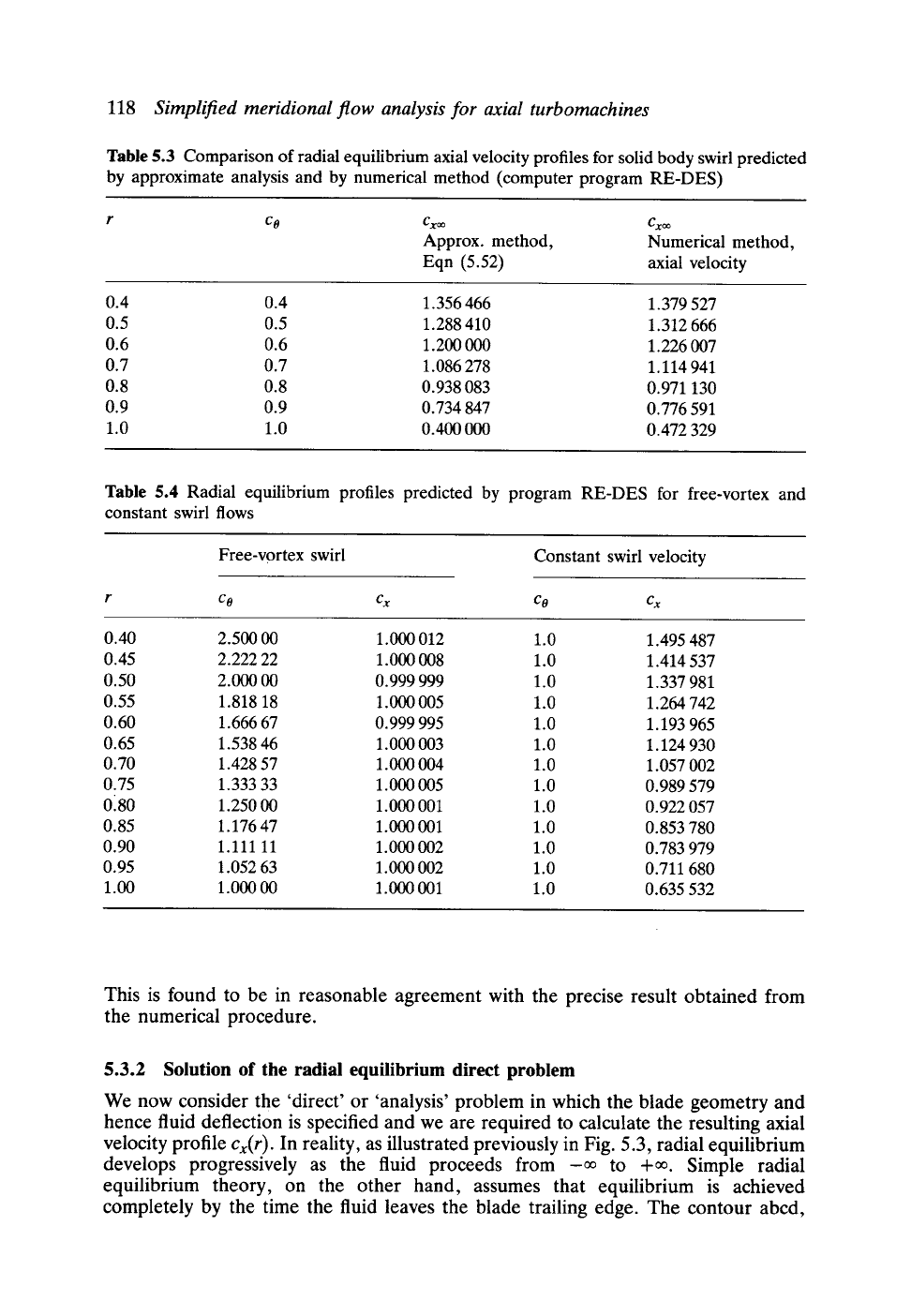
Table 5.3 Comparison of radial equilibrium axial velocity profiles for solid body swirl predicted
by approximate analysis and by numerical method (computer program RE-DES)
r co
Cxoo Cxoo
Approx. method, Numerical method,
Eqn (5.52) axial velocity
0.4 0.4 1.356 466 1.379 527
0.5 0.5 1.288 410 1.312 666
0.6 0.6 1.200 000 1.226 007
0.7 0.7 1.086 278 1.114 941
0.8 0.8 0.938 083 0.971 130
0.9 0.9 0.734 847 0.776 591
1.0 1.0 0.400 000 0.472 329
Table 5.4 Radial equilibrium profiles predicted by program RE-DES for free-vortex and
constant swirl flows
Free-vortex swirl
Constant swirl velocity
r c o c x Co cx
0.40 2.500 00 1.000 012 1.0 1.495 487
0.45 2.222 22 1.000 008 1.0 1.414 537
0.50 2.000 00 0.999 999 1.0 1.337 981
0.55 1.818 18 1.000 005 1.0 1.264 742
0.60 1.666 67 0.999 995 1.0 1.193 965
0.65 1.538 46 1.000 003 1.0 1.124 930
0.70 1.428 57 1.000 004 1.0 1.057 002
0.75 1.333 33 1.000 005 1.0 0.989 579
0180 1.250 00 1.000 001 1.0 0.922 057
0.85 1.176 47 1.000 001 1.0 0.853 780
0.90 1.111 11 1.000 002 1.0 0.783 979
0.95 1.052 63 1.000 002 1.0 0.711 680
1.00 1.000 00 1.000 001 1.0 0.635 532
This is found to be in reasonable agreement with the precise result obtained from
the numerical procedure.
5.3.2 Solution of the radial equilibrium direct problem
We now consider the 'direct' or 'analysis' problem in which the blade geometry and
hence fluid deflection is specified and we are required to calculate the resulting axial
velocity profile
Cx(r).
In reality, as illustrated previously in Fig. 5.3, radial equilibrium
develops progressively as the fluid proceeds from -oo to +oo. Simple radial
equilibrium theory, on the other hand, assumes that equilibrium is achieved
completely by the time the fluid leaves the blade trailing edge. The contour abcd,
5.3
Solution of the radial equilibrium equation
119
Cxl
73
,,,,...-
Vd
Cx2
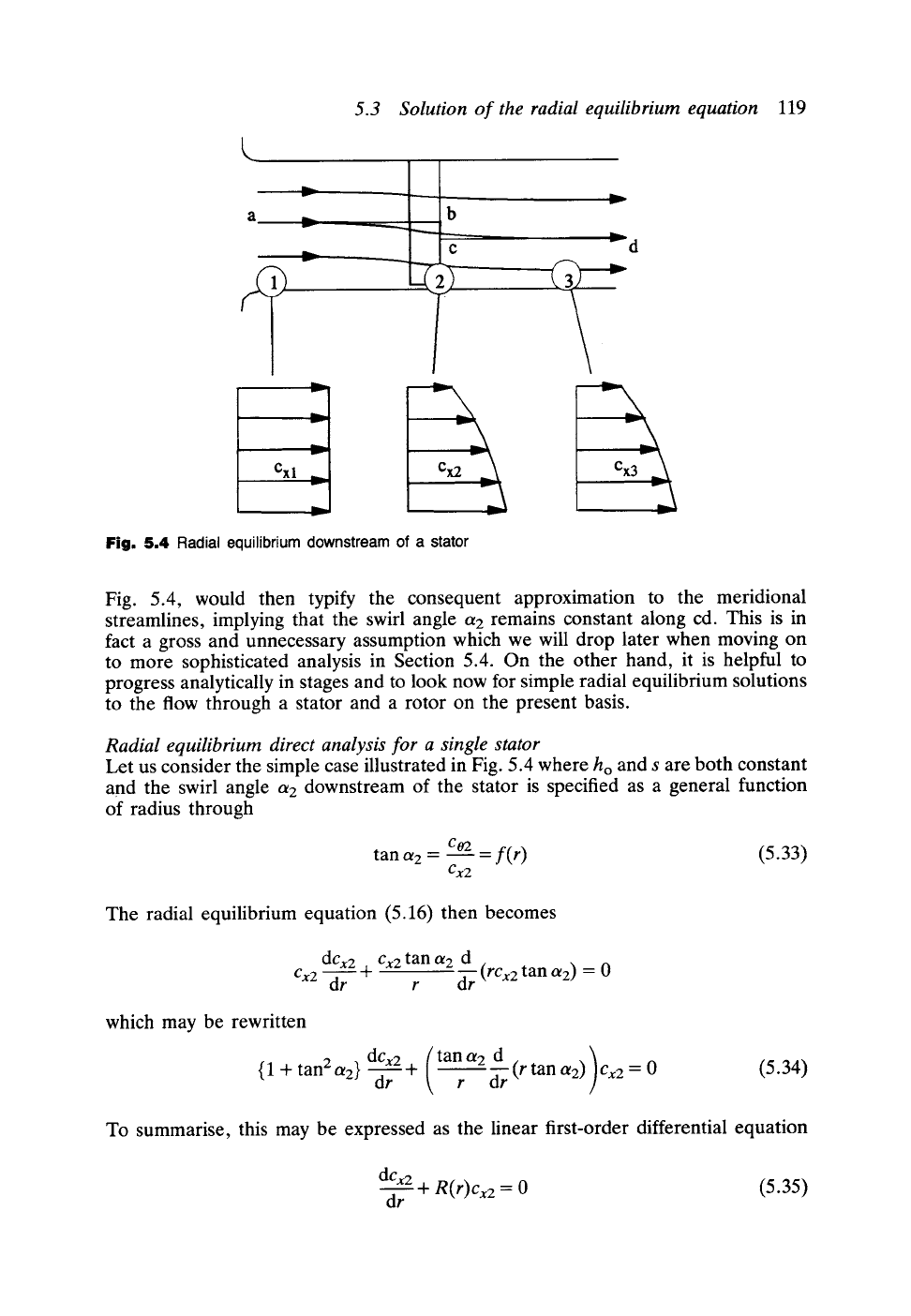
Fig. 5.4 Radial equilibrium downstream of a stator
Cx3"- 5
....--
Fig. 5.4, would then typify the consequent approximation to the meridional
streamlines, implying that the swirl angle a2 remains constant along cd. This is in
fact a gross and unnecessary assumption which we will drop later when moving on
to more sophisticated analysis in Section 5.4. On the other hand, it is helpful to
progress analytically in stages and to look now for simple radial equilibrium solutions
to the flow through a stator and a rotor on the present basis.
Radial equilibrium direct analysis for a single stator
Let us consider the simple case illustrated in Fig. 5.4 where ho and s are both constant
and the swirl angle a2 downstream of the stator is specified as a general function
of radius through
C02
tana2 = ~ = f(r) (5.33)
Cx2
The radial equilibrium equation (5.16) then becomes
dcx2
Cx2 --d-~-r +
Cx2
tan
O~ 2
d
r d--; (rCx2
tan a2) = 0
which may be rewritten
dcx2
{ 1 + tan 2
r162 -~r
tan ot 2
d )
+ (r tan a2)
Cx2
-- 0
(5.34)
r dr
To summarise, this may be expressed as the linear first-order differential equation
dcx_____g2 _
dr ~- R(r)Cxe
= 0 (5.35)
120 Simplified meridional flow analysis for axial turbomachines
where R(r) is a function of radius given by
R(r) =
tan ot 2
d (r
tan or2)
r dr
1 + tan 2 a 2
(5.36)
The general solution of Eqn (5.35) is given by
Cx2 = K exp (- f R(r) dr)
(5.37)
where the constant K must be determined from the continuity equation (5.20).
Example 5.5 Constant a z stator
Problem
Derive an expression for CxE/Cx downstream of a stator given that tan
Ot 2 --constant.
Solution
The function R(r), Eqn (5.36), now reduces to
1( tan2a2 ) = sin2a2 _p
R(r) = 1 + tan 20~
2 r --
where p = sin 20~
2.
Thus
f R(r) dr = In (r e)
and
exp (- f R(r) dr) = r -p
Equation (5.37) thus yields the solution
Cx2 =
Kr-P
Application of the continuity equation (5.20) then results in
I
rt
Cx 7r(r 2 - r 2) = 27rK r I -p dr
h
27rK
2-p
~[r2-p_ r2-p]
and hence the constant K is determined through
K = Cx(r2- r2)(1 -p/2)
r -P
5.3 Solution of the radial equilibrium equation
121
L
O3
(-
Cx2
O3
v
f
I__.
w02
I
C02
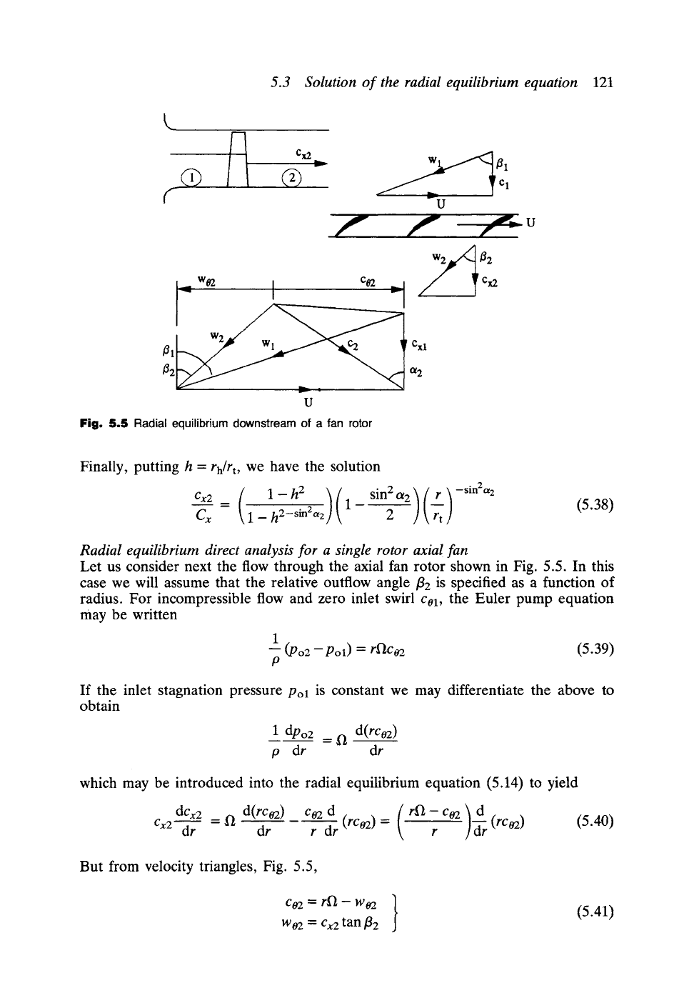
Fig. 5.5
Radial equilibrium downstream of a fan rotor
JJ ~ T cl
=.--
u
J.~ u
f r
w2~~2
Cxl
cz 2
Finally, putting h =
rh/rt,
we have the solution
Cx2 __ (1-h 2 )( sin2 a2) (~t
Cx
1-T
sin2a2 (5.38)
Radial equilibrium direct analysis for a single rotor axial fan
Let us consider next the flow through the axial fan rotor shown in Fig. 5.5. In this
case we will assume that the relative outflow angle/32 is specified as a function of
radius. For incompressible flow and zero inlet swirl
col,
the Euler pump equation
may be written
1
.2. (Po2 -- Pol) =
r12co2
(5.39)
P
If the inlet stagnation pressure Pol is constant we may differentiate the above to
obtain
1 dpo 2 = ~[~ d(rc02)
p dr dr
which may be introduced into the radial equilibrium equation (5.14) to yield
dcx2 d(rco2) co2d
( r[l- c02) d
Cx2T : ['~
dr r dr (rco2) = r -dr (rc~
(5.40)
But from velocity triangles, Fig. 5.5,
c~ = r~-- w ~ }
W o2 = Cx2
tan/32
(5.41)
122
Simplified meridional flow analysis for axial turbomachines
Introduction of these equations into Eqn (5.40) leads finally to the following
first-order linear differential equation"
dcx2
(tan
f12 d
{1 + tan 2
fiE} ~ "+"
r
dr
(r
tan f12) )
r
-"
21~ tan
f12
(5.42a)
which may be summarised as
dcx2
d----~ + fl(r)Cx2
= fz(r) (5.42b)
where the two functions of radius are given by
f1(r) = ( tan [32 d (r tan f12) ) 1
r dr 1 + tan 2/32
21~ tan
fiE
f2(r) = 1 + tan 2 fiE
(5.43)
The standard procedure for solution of Eqn (5.42) is to multiply throughout by
exp(ffl(r)dr)
anti then integrate with respect to radius, resulting in
ff2(r) (ffl(r)
dr) dr + K1
exp
Cx2
= (5.44)
exp(ffl(r)dr)
As for the previous example of the stator blade row, the constant K1 must be
determined from the continuity equation (5.20). We observe that the stator solution,
Eqn (5.37), is simply a subset of the above for the case when ~ = 0 and hence
f~(r)
= 0. For the free-vortex stator, on the other hand, since tan/32
=
K1/r,
fl(r)
is
also zero and Eqn (5.44) reduces as expected to
Cx2 = K1 = Cx.
Numerical solution of the direct problem for a fan rotor
Although a solution has been obtained above in closed analytic form, the integrals
in Eqn (5.44) would still in most cases need to be evaluated numerically. In view
of this a better strategy is to solve Eqn (5.42) numerically. Thus after integration the
solution may be expressed as
Cx2 =
L(r,
r + K1
(5.45)
where
I
r]
L(Fj, Cx2 ) -- ( -- Cx2fl (rj) d- f2(t]) }
dr
h
i
~- Ar 2 { - Cx2fl(ri) + f2(ri) }
i=1
(5.46)
where
f12
and thus
fl(ri)
and
f2(ri)
are specified at m equally spaced radii from rh
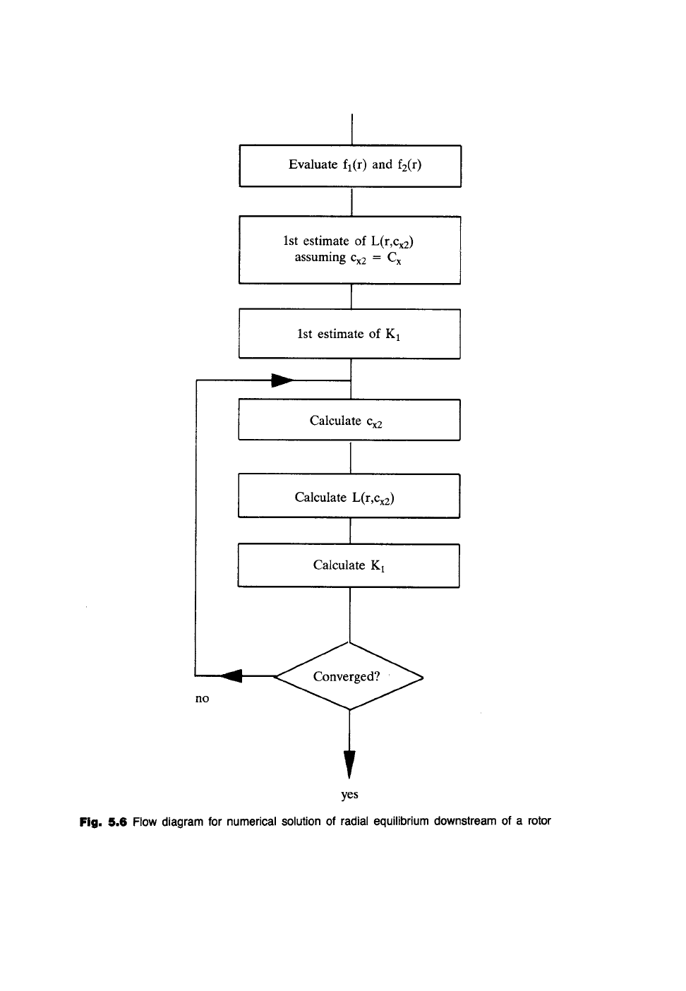
Evaluate fl(r) and f2(r)
1st estimate of
L(r,Cx2)
assuming
Cx2 = C x
1st estimate of K1
Calculate Cx2
Calculate L(r,Cx2)
!
Calculate K 1
no
yes
Fig. 5.6 Flow diagram for numerical solution of radial equilibrium downstream of a rotor