Lyons W.C. (ed.). Standard handbook of petroleum and natural gas engineering.2001- Volume 1
Подождите немного. Документ загружается.

Numerical Methods
85
therefore
1
AY
=
2
+By,)
and
YI
=
YO
+
'Y
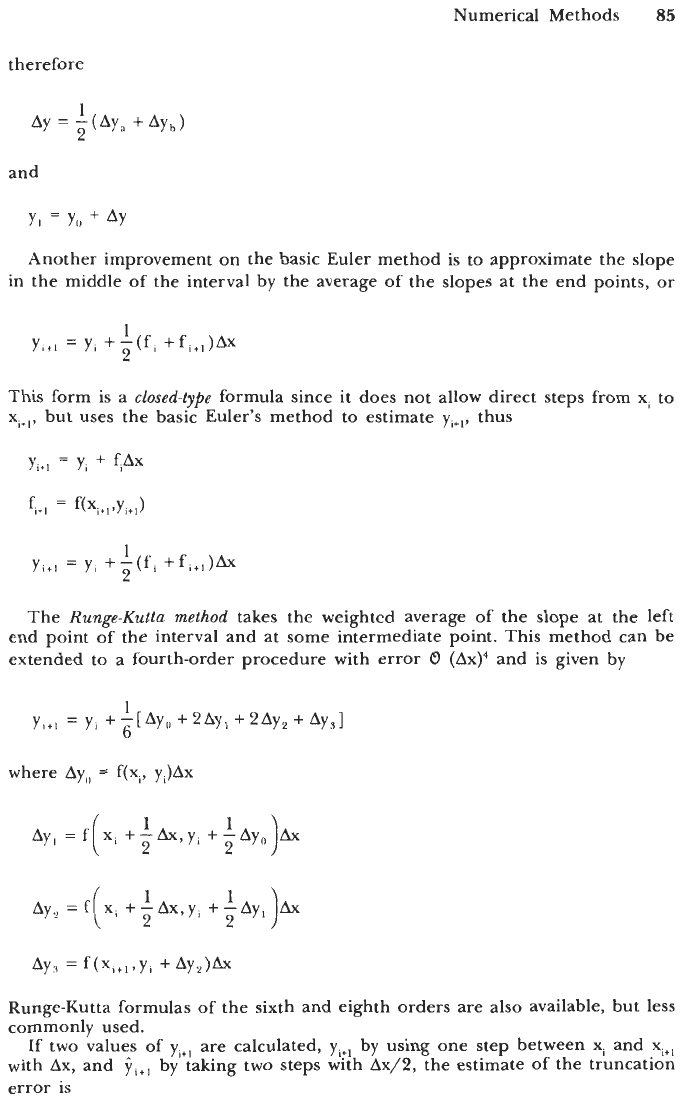
Another improvement on the basic Euler method is to approximate the slope
in the middle of the interval by the average of the slopes at the end points, or
This form
is
a
closed-type
formula since it does not allow direct steps from xi to
xirl, but uses the basic Euler's method to estimate
yitl,
thus
The
Runge-Kutta
method
takes the weighted average of the slope at the left
end point of the interval and at some intermediate point. This method can be
extended
to
a fourth-order procedure with error
0
AX)^
and is given by
where
Ayo
=
f(xi,
y,)Ax
Runge-Kutta formulas of the sixth and eighth orders are also available, but less
commonly used.
If
two values of
yi+l
are calculated,
yi+l
by using one step between xi and
xi+l
with Ax, and
y,,,
by taking two steps with Ax/2, the estimate of the truncation
error
is
86
Mathematics
Yi+l
-
Yicl
2-k
-
1
Ei+l
-
where k is the order
o
the expression (e.g., k
=
4
for the foregoing Runge-
Kutta formula). The step size can be adjusted to keep the error
E
below some
predetermined value.
The
Adams
Open
Formulas
are a class of multistep formulas such that the first-
order formula reproduces the Euler formula. The second-order Adams open
formula is given by
yitl
=
yi
+Ax
-fi
31
--fi&,]+O(Ax)'
[
22
This formula and the higher-order formulas are not self starting since they
require fi-l, fi-,, etc. The common practice is to employ a Runge-Kutta formula
of the same order to compute the first term(s) of
y,.
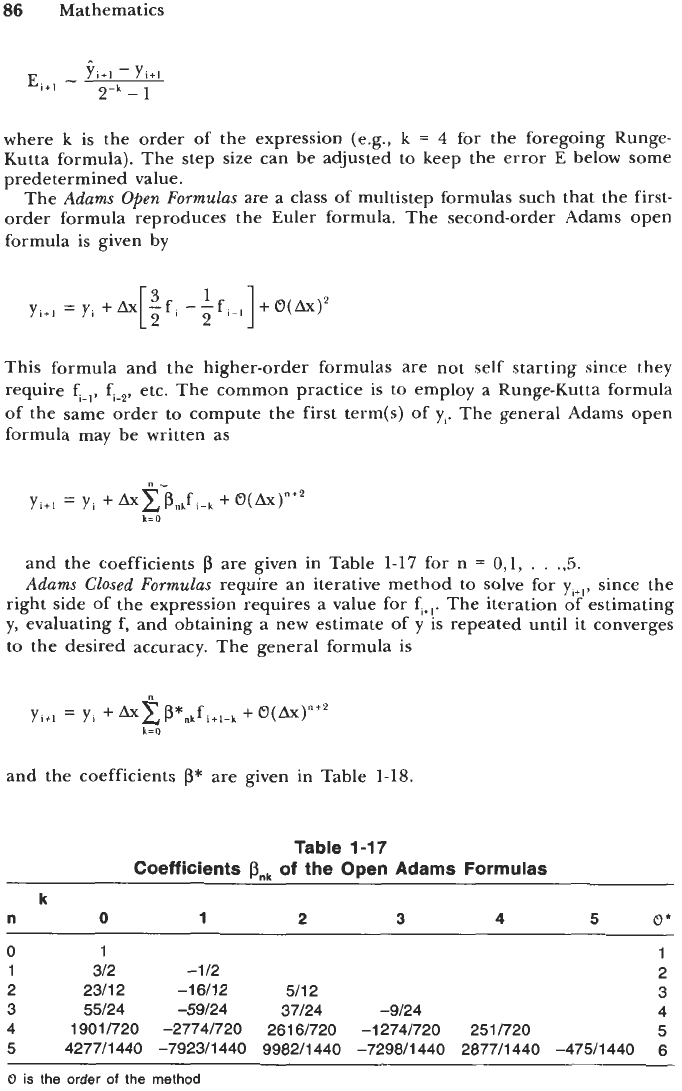
The general Adams open
formula may be written as
and the coefficients
p
are given in Table
1-17
for n
=
0,1,
. .
.,5.
Adams Closed Formulas
require an iterative method to solve for
Y,+~,
since the
right side of the expression requires a value for fi+,. The iteration of estimating
y,
evaluating f, and obtaining a new estimate of
y
is repeated until it converges
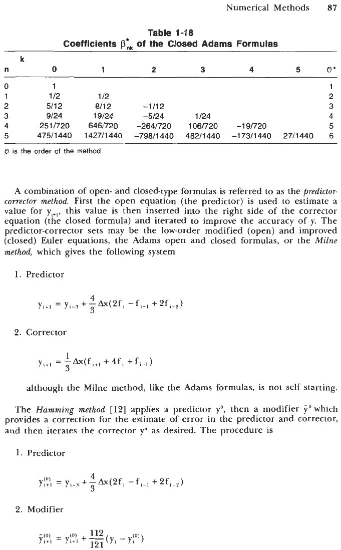
to the desired accuracy. The general formula
is
and the coefficients
p*
are given in Table
1-18.
Table
1-17
Coefficients
S,,
of
the Open
Adams
Formulas
k
n
0
1
2
3
4
5
o*
~ ~
0
1
1
1
312
-1
12 2
2 2311 2
-1
611 2 511 2 3
3
55/24 -59124 37/24 -9124
4
4 1901/720 -2774/720 261 61720
-1
2741720 251 1720
5
5 427711
440
-792311
440
99a211440 -729811
440
287711
440
-47511
440
6
0
is
the order
of
the method
Numerical Methods
87
Table
1-18
Coefficients
p*,,
of the Closed Adam Formulas
n
0
1 2
3
4
5
(7'
0
1
1
1 1
12 112 2
2 511 2 at1 2
-1
I1
2
3
3
9/24 19124 -5124 1124
4
4 2511720 646l720 -264l720 1061720 -191720 5
k
5 47511 440 142711 440 -79a11440 48211 440
-1
7311 440 2711 440 6
0
is
the order
of
the method
A combination of open- and closed-type formulas is referred to as the
predictor-
corrector method.
First the open equation (the predictor) is used to estimate a
value for
yi+l,
this value is then inserted into the right side of the corrector
equation (the closed formula) and iterated to improve the accuracy of
y.
The
predictor-corrector sets may be the low-order modified (open) and improved
(closed) Euler equations, the Adams open and closed formulas, or the
Milne
method,
which gives the following system
1.
Predictor
4
3
Yi+l
=
yi-5
+
-
W2f
-
f
i-1
+
2f
i-*)
2. Corrector
1
3
yj+,
=
-wfi+l
+4fi +fi&,)
although the Milne method, like the Adams formulas, is
not
self starting.
The
Humming method
[12] applies a predictor
yo,
then a modifier
i"
which
provides a correction for the estimate of error in the predictor and corrector,
and then iterates the corrector y" as desired. The procedure is
1. Predictor
4
Y!?,
=
y,-,+-k(2fi
3
-f,4 +2f,_,)
2.
Modifier
(0)
112
F!",:
=
Yi+l
+
-
(Y,
-
Y1O')
121
88
Mathematics
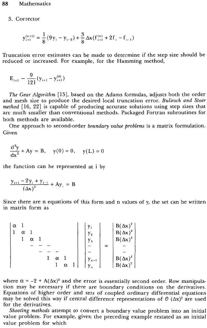
3.
Corrector
1
3
8
8
yp
=
-(9y, -yi-2)+-Ax(f:;;
+2f,
-f,-l)
Truncation error estimates can be made to determine
if
the step size should be
reduced
or
increased. For example, for the Hamming method,
The
Gear Algorithm
[15],
based on the Adams formulas, adjusts both the order
and mesh size to produce the desired local truncation error.
BuEirsch
and Stoer
method
[16,
221 is capable of producing accurate solutions using step sizes that
are much smaller than conventional methods. Packaged Fortran subroutines for
both methods are available.
One approach to second-order
boundary value probZems
is a matrix formulation.
Given
-+Ay=B,
d2Y
y(O)=O,
y(L)=O
dx2
the function can be represented at
i
by
Since there are n equations of this form and n values of y, the set can be written
in matrix form as
a1
1
a1
1
a1
---
---
la1
1
a1
YI
Y2
Y3
-
-
Y"-1
Y,
where
a
=
-2
+
A(Ax)~
and the error is essentially second order. Row manipula-
tion may be necessary
if
there are boundary conditions on the derivatives.
Equations of higher order and sets of coupled ordinary differential equations
may be solved this
way
if central difference representations
of
0
(Ax)' are used
for the derivatives.
Shooting methods
attempt to convert a boundary value problem into an initial
value problem. For example, given the preceding example restated as an initial
value problem for which
Numerical Methods
89
dY
y(0)
=
0
and
-(O)
=
U
dx
U is unknown and must be chosen
so
that y(L)
=
0.
The equation may be solved
as an initial value problem with predetermined step sizes
so
that xn will equal
L
at the end point. Since y(L) is a function of U, it will be denoted as y,(U)
and an appropriate value of U sought
so
that
Any standard root-seeking method that does not utilize explicitly the derivative
of the function may be employed.
Given two estimates of the root U,, and U,, two solutions of the initial value
problem are calculated, yL(Uoo) and yL(U,), a new estimate of
U
is obtained where
and the process is continued to convergence.
involving two independent variables:
There are three basic classes
of
second-order
partial differential equations
1.
Parabolic
2.
Elliptic
3.
Hyperbolic
where
@
=
$(x,y,u,au/ax,au/ay). Each class requires a different numerical
approach. (For higher-order equations and equations in three or more variables,
the extensions are usually straightforward.)
Given a parabolic equation of the form
90
Mathematics
with boundary conditions
u(a,y)
=
ua
uby)
=
u,,
U(X,O)
=
u,,
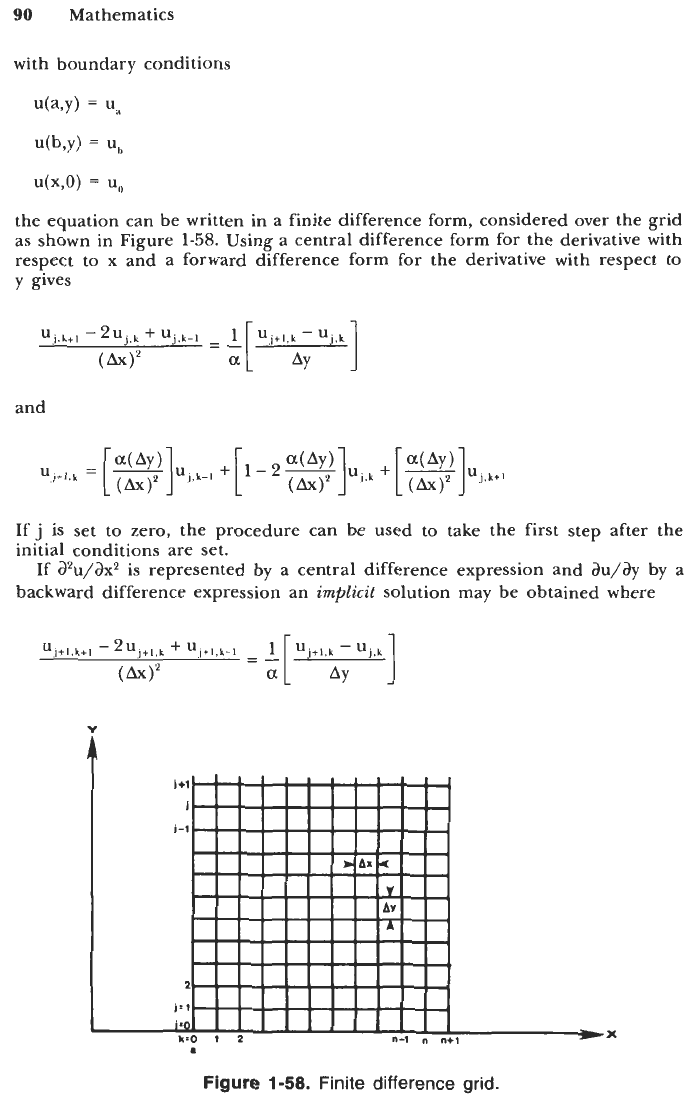
the equation can be written in a finite difference form, considered over the grid
as shown in Figure
1-58.
Using a central difference form for the derivative with
respect to x and a forward difference form for the derivative with respect to
y
gives
and
If
j
is set to zero, the procedure can be used to take the first step after the
initial conditions are set.
If
azu/ax2
is represented by a central difference expression and
h/ay
by a
backward difference expression an
implicit
solution may be obtained where
V
X
1
Figure
1-58.
Finite difference grid.
Numerical Methods
91
is
written for all k
=
1,2,
. .
.,
n.
A
set of n linear algebraic equations in n
unknowns is now defined, expressed in matrix form as
where
P
=
-
2
-
[(Ax)*]/[a(Ay)]
Q =
-
[(Ax)'l/[a(Ay)l
The
Crank-Nicholson method
is a special case of the formula
where
8 is
the degree of implicitness,
8
=
1 yields implicit representation,
8
=
1/2
gives Crank-Nicholson method, and
8
=
0,
the explicit representation.
8
2
1/2
is universally stable, while
8
<
1/2 is only conditionally stable.
Given a partial differential equation of the elliptic form
aZu
aZU
ax2
ay2
-+-=o
and a grid as shown in Figure 1-58, then the equation may be written in central
difference form at
(j,k)
as
and there are mn simultaneous equations in mn unknowns u,,!.
The most effective techniques for hyperbolic partial differential equations are
based on the
method ofcharacteristics
[19]
and
an
extensive treatment of this method
may be found in the literature of compressible fluid flow and plasticity fields.
Finite element methods
[20,2 11 have replaced finite difference methods in many
fields, especially in the area of partial differential equations. With the finite
element approach, the continuum is divided into a number of "finite elements"
that are assumed to be joined by a discrete number of points along their
boundaries.
A
function is chosen to represent the variation of the quantity over
each element in terms of the value
of
the quantity at the boundary points.
Therefore a set of simultaneous equations can be obtained that will produce a
large, banded matrix.
92
Mathematics
The three primary advantages of the finite element approach over finite
difference methods are
[9]:
1.
Easy handling of irregularly shaped regions.
2.
Variation in size of elements over a region, allowing smaller elements where
strong variations occur.
3.
Larger elements can produce comparable accuracy to smaller mesh elements
of a finite difference grid, which is especially useful in handling elliptic
partial differential matrices.
Other methods for solving PDE's include Monte Carlo, spectral, and varia-
tional. Spectral methods in particular converge more rapidly than finite dif-
ference methods, but do not handle problems involving irregular geometries or
discontinuities well.
APPLIED STATISTICS
See References
23-28
for additional information.
A
discrete random variable
is one that may take on only distinct, usually integer,
values.
A
continuous random variable
is one that may take on any value within a
continuum of values.
Moments
The moments describe the characteristics of a sample or distribution function.
The
mean,
which locates the average value on the measurement axis, is the first
moment of values measured about the origin. The mean is denoted by
p
for
the population and
X
for the sample and is given for a continuous random
variable by
For a discrete random variable, the mean is given by
and if each observation is given equal weight, f(X)
=
l/n and
-
1"
x
or
p
=
-Cxi
n
i=l
The
variance
is the second moment about the mean and indicates the closeness
of values
to
the mean. It is denoted by
o2
(population) or
Sz
(sample) and is
given for a continuous random variable by
Applied Statistics
93
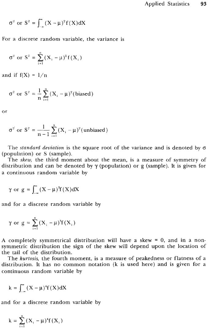
For a discrete random variable. the variance
is
and
if
f(X)
=
l/n
&J
or
S?
- -
-
'
t(X, -F)'(biased)
n
i=l
or
The
standard deviation
is the square root of the variance and is denoted by
Q
(population) or
S
(sample).
The
skew,
the third moment about the mean, is a measure of symmetry
of
distribution and can be denoted by
y
(population) or
g
(sample). It is given for
a continuous random variable by
and for a discrete random variable by
A
completely symmetrical distribution will have a skew
=
0,
and in a non-
symmetric distribution the sign of the skew will depend upon the location of
the tail of the distribution.
The
kurtosis,
the fourth moment, is
a
measure of peakedness or flatness of a
distribution. It has no common notation
(k
is used here) and is given for a
continuous random variable by
k
=
Jm
(X
-
~)~f(X)dx
-m
and for a discrete random variable by
94
Mathematics
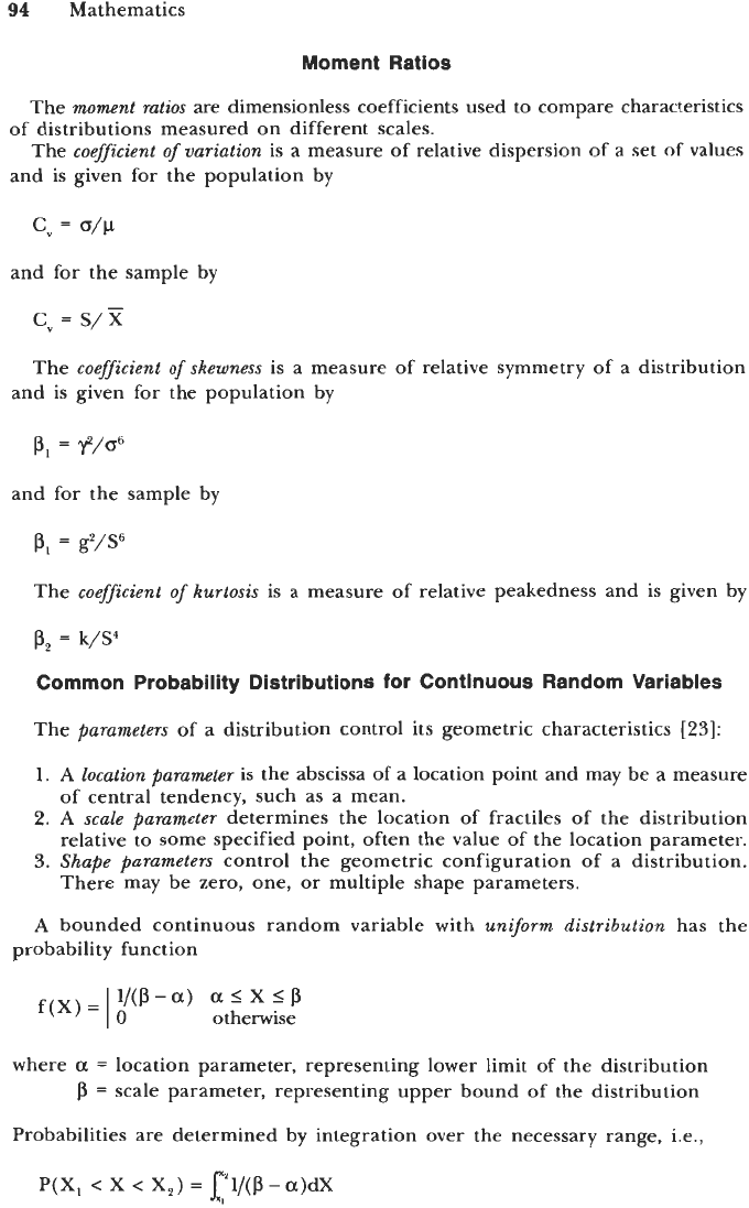
Moment Ratios
The
moment ratios
are dimensionless coefficients used to compare characteristics
The
coefficient of variation
is a measure of relative dispersion of a set of values
of distributions measured on different scales.
and is given for the population by
and for the sample by
C"
=
s/x
The
coefficient of skewness
is a measure of relative symmetry of a distribution
and is given for the population by
and for the sample by
The
coefficient of kurtosis
is a measure of relative peakedness and is given by
P,
=
k/S4
Common Probability Distributions for Continuous Random Variables
The
parameters
of a distribution control its geometric characteristics
[23]:
1.
A
location parameter
is the abscissa of a location point and may be a measure
of central tendency, such as a mean.
2.
A
scale parameter
determines the location of fractiles of the distribution
relative to some specified point, often the value of the location parameter.
3.
Shape parameters
control the geometric configuration of a distribution.
There may be zero, one, or multiple shape parameters.
A
bounded continuous random variable with
uniform distribution
has the
probability function
f(X)
=
I
$'(P-a)
a
<
X
<
P
otherwise
where
a
=
location parameter, representing lower limit of the distribution
P
=
scale parameter, representing upper bound of the distribution
Probabilities are determined by integration over the necessary range, Le.,
P(X,
<
x
<
X,)
=
p/(p
-
a)dX
I